Calculations in Star Charts
Yuk Tung Liu
First draft: 2018-07-10, last major update: 2025-07-08
Note: This is an HTML version of this pdf file. Use the pdf if your browser doesn't render some texts and equations correctly. In case of any discrepancy between the two versions, the pdf version shall prevail.
This document lists the equations used in the calculations on the webpages local star charts and equatorial star charts.
The local star chart page uses the computer's clock to obtain the current local time and then uses it to calculate the local sidereal times and plot star charts on two locations. The two default locations are at longitude 98.6174°W, latitude 29.5866°N (UT San Antonio, TX, USA) and at longitude 98.6174°W, latitude 30°S. Sidereal times and star charts at other locations and times can be obtained by clicking the Locations and Times button at the top of the page and filling in the form.
The two default locations can be changed by modifying the init_cont() function in the file sidereal.js. The variables place1 is the name of location 1, long1 is the longitude of location 1 in degrees (negative to the west of Greenwich and positive to the east of Greenwich), lat1 is the (geodetic) latitude of location 1 in degrees (negative in the southern hemisphere and positive in the northern hemisphere). The javascript object tz1 stores the time zone information of location 1: tz1.tz is the time zone offset in minutes, i.e. the difference between the local time and UT (positive if the local time is behind UT and negative if the local time is ahead of UT); tz1.tzString stores the string "GMT±hhmm", where ±hhmm provides the time zone information. Currently, tz1 is set according to the information obtained from the computer clock. The variables place2, long2, lat2, and tz2 store the corresponding information for location 2.
Location 1 can also be determined from user's IP address using the server on http://ip-api.com/. This option is currently disabled. It can be enabled by setting the variable iplookup to true inside function init() in the file sidereal.js.
Sidereal time is defined as the hour angle of the vernal equinox. Thus, it depends on the observation point and how the vernal equinox and equator are defined. The celestial equator and equinoxes move with respect to an inertial frame because of the tidal torques of the Moon, Sun and planets on the oblate Earth. When the effect of precession, but not nutation, is included, the resulting equator and equinoxes are called the mean equator and equinoxes. When both precession and nutation are included, the resulting equator and equinoxes are called the true equator and equinoxes.
The mean sidereal time is the hour angle of the mean vernal equinox of date, i.e. it is the angle, measured along the mean equator, from the observer's meridian to the great circle that passes through the mean vernal equinox and the mean celestial poles. The apparent sidereal time is the hour angle of the true vernal equinox of date. Apparent sidereal time minus mean sidereal time is the equation of the equinoxes.
The Greenwich sidereal time (GST) is the sidereal time measured at Greenwich. In particular, Greenwich mean sidereal time (GMST) is the mean sidereal time at Greenwich. Greenwich apparent sidereal time (GAST) is the apparent sidereal time at Greenwich. The local sidereal time (LST) is related to the GST by
$$ {\rm LST = GST} + \lambda , \label{eq:LST} $$where $\lambda$ is the longitude of the observation point, positive if it is to the east of Greenwich and negative if it is to the west of Greenwich.
Universal Time (UT) is a time standard based on Earth's rotation with respect to the Sun. There are several versions of universal time. The most commonly used are UT1 and the Coordinated Universal Time (UTC).
Prior to 1 January 2003, UT1 was defined by a specified function of GMST. Starting from 1 January 2003, UT1 is defined as a linear function of the Earth rotation angle (ERA). ERA is the modern version of the Greenwich sidereal time. It is defined as the angle measured along the true equator between Celestial Intermediate Origin (CIO) and the Terrestrial Intermediate Origin (TIO). CIO is the modern version of the vernal equinox and TIO is the modern version of the Greenwich meridian.
Recall that GMST is the hour angle of the mean vernal equinox measured from the Greenwich meridian. The mean vernal equinox moves with respect to an inertial frame because of precession. The dominant component is the westward motion of 50.3" per year. CIO, on the other hand, is defined to be non-rotating. As the true equator moves, the path of the CIO in space is such that the point has no instantaneous east-west velocity along the true equator. TIO is a modern version of the prime meridian on Earth. Unlike the Greenwich meridian, TIO is not fixed on the geographic surface on Earth. It is defined kinematically such that there is no component of polar motion about the pole of rotation. To sum up, CIO replaces the moving equinox as the origin of the celestial coordinate system; TIO replaces the Greenwich meridian as the origin of the longitude; and ERA replaces GST as a measure of Earth's rotation.
As explained in Section 3.2 of Explanatory Supplement to the Astronomical Almanac , Earth's rotation is not uniform. There are three kinds of variations in Earth's rotation: (1) steady deceleration, (2) random fluctuations, and (3) periodic changes. Measurements show that the length of a day is on average increasing at a rate of 1.7 ms per century. The tidal friction from the Moon and Sun causes the increase in the length of a day by 2.3 ms per century. The 0.6 ms per century discrepancy between the measured deceleration and the deceleration caused by the tidal friction is possibly associated with changes in the figure of the Earth caused by post-glacial rebound or with deep ocean dissipation. The random fluctuations in Earth's rotation is probably caused by the interaction of the core and mantle of the Earth. The periodic changes in Earth's rotation is mainly caused by meteorological effects and periodic variations caused by luni-solar tides.
Because of the random components in the rotation of the Earth, accurate value of ERA must be obtained from observations. It is determined by Very Long Baseline Interferometry (VLBI) measurements of selected extra-galactic radio sources, mostly quasars, and interpolated by tracking of GPS satellites. Once the ERA, $\theta$, is measured, UT1 is defined by the linear equation (IAU Resolution B1.8)
$$ \theta(D_U) = 2\pi (0.7790572732640 + 1.00273781191135448 D_U) , \label{def:UT1} $$where $D_U = {\rm Julian UT1 date} - 2451545.0$. Note that UT1 is defined by equation \eqref{def:UT1}.
The nonuniformity of UT1 is inconvenient for many applications. As a result, UTC is introduced to approximate UT1. UTC is defined by two components: International Atomic Time (TAI) and UT1. TAI is a weighted average of the time kept by over 400 atomic clocks in over 50 national laboratories worldwide. Each second in a TAI is one SI second, defined as the duration of 9,192,631,770 periods of the radiation corresponding to the transition between the two hyperfine levels of the ground state of the caesium-133 atom. UTC is defined to be TAI plus an integral number of seconds. The duration of one second in UTC is therefore exactly equal to one SI second. Leap seconds are added to ensure approximate agreement with UT1: |UTC-UT1| < 0.9s. As of today (2025-07-08), a total of 27 leap seconds have been inserted since the system of adjustment was implemented in 1972. The most recent leap second occurred on December 31, 2016 at 23:59:60 UTC.
Civil time is related to UTC by a UTC offset. A UTC offset is a multiple of 15 minutes, and the majority of offsets are in whole hours. On our webpages, civil (local) times are expressed as GMT±hhmm, where ±hhmm indicates the UTC offset. For example, GMT-0600 means the local time is UTC - 6 hours; GMT+0545 means the local time is UTC + 5 hours and 45 minutes.
From the 17th century to the late 19th century, planetary ephemerides were calculated using time scales based on Earth's rotation. It was assumed that Earth's rotation was uniform. As the precision of astronomical measurements increased, it became clear that Earth's rotation is not uniform. Ephemeris time (ET) was introduced to ensure a uniform time for ephemeris calculations. It was defined by the orbital motion of the Earth around the Sun instead of Earth's spin motion. However, a more precise definition of times is required when general relativistic effects need to be included in ephemeris calculations.
In general relativity, the passage of time measured by an observer depends on the spacetime trajectory of the observer. To calculate the motion of objects in the solar system, the most convenient time is a coordinate time, which does not depend on the motion of any object but is defined through the spacetime metric. In the Barycentric Celestial Reference System (BCRS), the spacetime coordinates are $(t,x^i)$ $( i=1,2,3)$. Here the time coordinate $t$ is called the barycentric coordinate time (TCB). The spacetime metric for the solar system can be written as [see Eq. (2.38) in Explanatory Supplement to the Astronomical Almanac]
$$ ds^2 = -\left( 1 - \frac{2w}{c^2} + \frac{2w^2}{c^4}\right) d(ct)^2 - \frac{4 w_i}{c^3} d(ct) dx^i + \delta_{ij}\left[ 1 + \frac{2w}{c^2} + O(c^{-4})\right] dx^i dx^j , \label{eq:BCRS_metric} $$where sum over repeated indices is implied. The scalar potential $w$ reduces to the Newtonian gravitational potential $-\Phi$ in the Newtonian limit, where
$$ \Phi(t,\boldsymbol{x}) = -G\int d^3x' \frac{\rho(t,\boldsymbol{x'})}{|\boldsymbol{x}-\boldsymbol{x'}|} $$and $\rho$ is the mass density. The vector potential $w_i$ satisfies the Poisson equations with the source terms proportional to the momentum density.
TCB can be regarded as the proper time measured by an observer far away from the solar system and is stationary with respect to the solar system barycenter. The equations of motion for solar system objects can be derived in the post-Newtonian framework. The result is a system of coupled differential equations and can be integrated numerically. In this framework, TCB is the natural choice of time parameter for planetary ephemerides. However, since most measurements are carried out on Earth, it is also useful to set up a coordinate system with origin at the Earth's center of mass. In the geocentric celestial reference system (GCRS), the spacetime coordinates are $(T,X^i)$, where the time parameter $T$ is called the geocentric coordinate time (TGC). GCRS is comoving with Earth's center of mass in the solar system, and its spatial coordinates $X^i$ are chosen to be kinematically non-rotating with respect to the barycentric coordinates $x^i$. The coordinate time TCG is chosen so that the spacetime metric has a form similar to equation \eqref{eq:BCRS_metric}. Since GCRS is comoving with the Earth, it is inside the potential well of the solar system. As a result, TCG elapses slower than TCB because of the combined effect of gravitational time dilation and special relativistic time dilation. The relation between TCB and TCG is given by [equation (3.25) in Explanatory Supplement to the Astronomical Almanac]
$$ {\rm TCB} - {\rm TCG} = c^{-2} \left[ \int_{t_0}^t \left( \frac{v_e^2}{2} - \Phi_{\rm ext}(\boldsymbol{x_e}) \right) dt + \boldsymbol{v_e} \cdot (\boldsymbol{x}-\boldsymbol{x_e})\right] + O(c^{-4}) , \label{eq:TCG} $$where $\boldsymbol{x_e}$ and $\boldsymbol{v_e}$ are the barycentric position and velocity of the Earth's center of mass, and $\boldsymbol{x}$ is the barycentric position of the observer. The external potential $\Phi_{\rm ext}$ is the Newtonian gravitational potential of all solar system bodies apart from the Earth. The constant time $t_0$ is chosen so that TCB=TCG=ET at the epoch 1977 January 1, 0h TAI.
Since the definition of TCG involves only external gravity, TCG's rate is faster than TAI's because of the relativistic time dilation caused by Earth's gravity and spin. The terrestrial time (TT), formerly called the terrestrial dynamical time (TDT), is defined so that its rate is the same as the rate of TAI. The rate of TT is slower than TCG by $-\Phi_{\rm eff}/c^2$ on the geoid (Earth surface at mean sea level), where $\Phi_{\rm eff}=\Phi_E - v^2_{\rm rot}/2$ is the sum of Earth's Newtonian gravitational potential and the centrifugal potential. Here $v_{\rm rot}$ is the speed of Earth's spin at the observer's location. The value of $\Phi_{\rm eff}$ is constant on the geoid because the geoid is defined to be an equipotential surface of $\Phi_{\rm eff}$. Thus, $d {\rm TT}/d {\rm TCG} = 1-L_G$ and $L_G$ is determined by measurements to be $L_G=6.969290134\times 10^{-10}$. Therefore, TT and TCG are related by a linear relationship [equation (3.27) in Explanatory Supplement to the Astronomical Almanac]:
$$ {\rm TT} = {\rm TCG} - L_G ({\rm JD}_{\rm TCG} - 2443144.5003725) \cdot 86400 {\rm s} , \label{def:TT} $$where JDTCG is TCG expressed as a Julian date (JD). The constant 2443144.5003725 is chosen so that TT=TCG=ET at the epoch 1977 January 1 0h TAI (JD = 2443144.5003725). Since the rate of TT is the same as that of TAI, the two times are related by a constant offset:
$$ {\rm TT} = {\rm TAI} + 32.184 {\rm s} .$$The offset arises from the requirement that TT match ET at the chosen epoch.
TCB is a convenient time for planetary ephemerides, whereas TT can be measured directly by atomic clocks on Earth. The two times are related by equations \eqref{eq:TCG} and \eqref{def:TT} and must be computed by numerical integration together with the planetary positions. TT is therefore not convenient for planetary ephemerides. The barycentric dynamical time (TDB) is introduced to approximate TT. It is defined to be a linear function of TCB and is set as close to TT as possible. Since the rates of TT and TCB are different and are changing with time, TT cannot be written as a linear function of TCB. The best we can do is to set the rate of TDB the same as the rate of TT averaged over a certain time period, so that there is no long-term secular drift between TT and TDB over that time period. The resulting deviation between TDB and TT has components of periodic variation caused by the eccentricity of Earth's orbit and the gravitational fields of the Moon and planets. TDB is now defined by the IAU 2006 resolution 3 as
$$ {\rm TDB} = {\rm TCB} - L_B ({\rm JD_{TCB}} - 2443144.5003725)\cdot 86400 {\rm s} - 6.55\times 10^{-5} {\rm s} ,$$where $L_B= 1.550519768\times 10^{-8}$ and ${\rm JD_{TCB}}$ is TCB expressed as a Julian date (JD). The value of $L_B$ can be regarded as $1-d {\rm TT}/dt$ averaged over a certain time period.
TDB is a successor of ET. It is now used by the Jet Propulsion Laboratory to calculate high-precision ephemerides of the Sun, Moon and planets. The relationship between TT and TDB can be written as (Figure 3.2 in Explanatory Supplement to the Astronomical Almanac]
\begin{align} {\rm TDB} &= {\rm TT} + 0.001658{\rm s} \sin(g + 0.0167\sin g) \nonumber \cr & + \mbox{ lunar and planetary terms of order } 10^{-5} {\rm s} \nonumber \cr & + \mbox{ daily terms of order} 10^{-6} {\rm s} , \end{align}where $g$ is the mean anomaly of Earth in its orbit (and hence $g+0.0167\sin g$ is the approximate value of the eccentric anomaly since 0.0167 is Earth's orbital eccentricity). A more detailed expression is given by equation (2.6) in . The difference between TDB and TT remains under 2 ms for several millennia around the present epoch. Hereafter, TT and TDB will be used interchangeably.
ΔT is defined to be the difference between TT and UT1:
$$ \Delta T = {\rm TT - UT1} , \label{def:DeltaT} $$Since ${\rm UTC = TAI} - \Delta ({\rm AT})$ and ${\rm TT = TAI + 32.184 s}$,
$$ {\rm TT - UTC = 32.184 s} + \Delta ({\rm AT}) ,$$where Δ(AT)=10s + total number of leap seconds added to UTC since 1972. Computer's clocks are mostly based on UTC plus an offset. The difference between UTC and UT1 is ignored here. It should be noted that almost all computations involving the Sun, Moon, planets and stars are based on TT. The only exception is computing the sidereal time, in which there is a term linear in UT1 by definition.
Because of the irregularity of Earth's rotation, UT1 and ΔT must be determined by observations. Future values of ΔT may be extrapolated from the current data, but the uncertainty grows with time. We also don't have accurate observational data for ΔT before 1600. ΔT on our webpages are calculated using the fitting and extrapolation formulae by Stephenson et al (2016) and Morrison et al (2021) (see also the HMNAO Earth rotation webpage for a summary). Specifically, values of ΔT from -720 to 2025 are computed using their spline fit cubic polynomials, but the coefficients after 2012 have been modified to extend the fitting formulae to 2025 (their original formulae are fitted to 2019). Outside this range ΔT is extrapolated by integrating their long-term lod function:
\begin{align} t &= (y - 1825)/100 \ \ , \ \ f(y) = 31.4115t^2 + 284.8436 \cos [2\pi(t + 0.75)/14] , \\ \Delta T &= \left\{ \begin{array}{cc} c_1 + f(y) & \mbox{ for } y \lt -720 \\ c_2 + f(y) & \mbox{ for } y \gt 2025 \end{array} \right. \ \ , \end{align}where $y$ is year, $t$ is the number of centuries from 1825, $c_1=1$ and $c_2=-150.568$. The formula gives ΔT in seconds. The values of $c_1$ and $c_2$ are chosen to make ΔT continuous at y = -720 and y = 2025. For a given Julian date number JD, y may be calculated by $y = (JD-2451544.5)/365.2425 + 2000$ for JD ≥ 2299160.5 and $y = (JD+0.5)/365.25 - 4712$ for JD < 2299160.5. The value 2299160.5 is the JD at 0h on October 15, 1582, which was the date when the Western calendar was switched from the Julian calendar to Gregorian calendar.
These fitting and extrapolation formulae are from the most recent study of ΔT that I am aware of. I have employed these new formulae on my eclipse website. I have also created a GitHub repository to provide python functions to calculate ΔT and to provide error estimates.
Our webpages use the Gregorian calendar on and after October 15, 1582 (JD 2299160.5) and Julian calendar before that day. Note that October 4, 1582 (JD 2299159.5) was followed by October 15, 1582 because of the Gregorian calendar reform. Our webpages take this into account. However, it should be noted that only only Spain, Portugal, France, Poland, Italy, Catholic Low Countries and colonies adopted the new calendar in 1582. Over the next three centuries, the Protestant and Eastern Orthodox countries also adopted the new calendar, with Greece being the last European country to adopt the calendar in 1923. Proleptic Julian calendar is used for years before 8 CE (CE = common era).
Conversion between Julian date and calendar date is implemented by the algorithm in Section 2.2 of the book Astronomy on the Personal Computer by O. Montenbruck and T. Pfleger, 4th edition, Springer 2000 (corrected fourth printing 2009).
As mentioned in Section 3, the solar system metric can be written in the Barycentric Celestial Reference System (BCRS). The origin of the BCRS spatial coordinates is at the solar system barycenter, i.e. the center of mass of the solar system. However, BCRS is a dynamical concept. The statement of "we use BCRS" in general relativity is equivalent to the statement "we use barycentric inertial coordinates" in Newtonian mechanics. BCRS does not define the orientation of the coordinate axes.
The International Celestial Reference System (ICRS) is a kinematical concept. Its origin is at the solar system barycenter. The ICRS axes are intended to be fixed with respect to space. They are determined based on hundreds of extra-galactic radio sources, mostly quasars, distributed around the sky. The ICRS axes are aligned with the equatorial system based on the J2000.0 mean equator and equinox to within 17.3 milliarcseconds. The $x$-axis of the ICRS points in the direction of the mean equinox of J2000.0. The $z$-axis points very close to the mean celestial north pole of J2000.0, and the $y$-axis is 90° to the east of the $x$-axis on the ICRS equatorial plane. So the ICRS is a right-handed rectangular coordinate system. The ICRS can be transformed to the equatorial system of J2000.0 by the frame bias matrix. However, since the difference between the two systems is tiny, I will not distinguish them.
It is assumed that the distant quasars and extragalactic radio sources do not rotate with respect to asymptotically flat reference systems like BCRS. In principle this assumption should be checked by testing if the motion of the solar system objects is compatible with the equation of motion based on BCRS, with no Coriolis and centrifugal forces. So far no deviations have been noticed.
However, it is expected that the extra-galactic radio sources should show a secular aberration drift caused by the rotation of the solar system barycenter around the center of Milky Way, and this drift was detected by analyzing decades of the very long baseline interferometry (VLBI) data (see Titov, Lambert & Gontier 2011). The magnitude of the drift is about 6 micro arcseconds per year, which agrees with the prediction. This effect will need to be taken into account in the future as measurement accuracies continue to improve.
Given the ICRS coordinates $(x,y,z)$ of an object, the ICRS right ascension $\alpha$ and declination $\delta$ are defined by the relation
$$ x = r \cos \alpha \cos \delta \ \ , \ \ y = r \sin \alpha \cos \delta \ \ , \ \ z = r \sin \delta , $$where $r=\sqrt{x^2+y^2+z^2}$. Hence $\alpha = \tan^{-1} (y/x)$ and $\delta = \sin^{-1}(z/r)$. The quadrant of $\alpha$ has to be determined appropriately from $x$ and $y$. Hereafter, I will write $\alpha = {\rm arg}(x+iy)$ to indicate that an appropriate quadrant should be used. Here ${\rm arg}(z)$ denotes the argument of a complex number $z$. Any complex number $z=x+iy$ can be written in the polar form $z=|z| e^{i\theta}$ and ${\rm arg}(z)$ is defined to be $\theta$. Thus, given a pair $(x,y)$, ${\rm arg}(x+iy)\ {\rm mod}\ 2\pi$ is unique. In the code, the function atan2() is used in favor of atan() since the quadrant is taken care of by atan2() automatically.
The origin of Geocentric Celestial Reference System (GCRS) is at the center of mass of the Earth. Ignoring general relativistic correction, the GCRS spatial coordinates $X^i$ are related to the BCRS spatial coordinates $x^i$ by
$$ X^i = x^i - x^i_E , \label{eq:GCRSX} $$where $x^i_E$ are the BCRS coordinates of Earth's center of mass. Relativistic correction adds terms of order $(v_E/c)^2 \sim 10^{-8}$, which I ignore. Like BCRS, GCRS is a dynamical concept. In the following, I will also use GCRS to refer to the coordinate system whose origin is at the geocenter and whose axes are oriented to the same directions as those of the ICRS.
The GCRS right ascension $\alpha$ and declination $\delta$ are defined in a similar way as the ICRS counterparts:
$$ X = R \cos \alpha \cos \delta \ \ , \ \ Y = R \sin \alpha \cos \delta \ \ , \ \ Z = R \sin \delta , \label{eq:GCRScoord} $$where $R=\sqrt{X^2+Y^2+Z^2}$.
Heliocentric coordinates are similar to the barycentric coordinates, except that the origin is located at the center of mass of the Sun. They are related to the barycentric coordinates by
$$ x^i_{\rm helio} = x^i - x^i_{\odot} ,$$where $x^i_{\odot}$ are the barycentric coordinates of the Sun's center of mass. Heliocentric coordinates are primarily used in the computation of planetary positions. Since the Sun contains 99.86% of the mass in the solar system, the solar system barycenter is very close to the Sun's center of mass.
The orientation of the coordinate axes described in Section 6 are fixed in space. This is convenient for describing the positions of stars and planets. However, observations are made on Earth's surface, which is rotating. The transformation between the celestial coordinate systems and the horizontal coordinate system centered on the observer involves taking into account Earth's rotation and the orientation of Earth's spin axis.
Earth's spin axis changes its orientation in space because of luni-solar and planetary torques on the oblate Earth. Earth's spin axis also moves relative to the crust. This is called the polar motion.
The motion of Earth's spin axis is composed of precession and nutation. Precession is the components that are aperiodic or have periods longer than 100 centuries. Nutation is the components that are of shorter periods and its magnitude is much smaller. Motion with periods shorter than two days cannot be distinguished from components of polar motion arising from the tidal deformation of the Earth. They are considered as components of polar motion. Therefore, nutation is defined as the periodic components in the motion of Earth's spin axis with periods longer than two days but shorter than about 100 centuries.
The major component of precession is the rotation of Earth's spin axis about the ecliptic pole with a period of about 26,000 years. This causes the vernal equinox to move westward by 50.3" per year. The principal period of nutation is 18.6 years, which is caused by the Moon's orbital plane precessing around the ecliptic. The amplitude of nutation is about 9". The amplitude of the polar motion is about 0.3".
In addition, the orbital plane of the Earth around the Sun also moves slowly because of planetary perturbation. Hence the ecliptic moves slowly in space. This is called the precession of the ecliptic, to be distinguished from the precession of the equator. Precession of the equator was formerly called the luni-solar precession, and precession of the ecliptic was formerly called the planetary precession. They are renamed because the terminologies are misleading. Planetary perturbation also contributes to the precession of the equator, although the magnitude is much smaller.
I do not include polar motion on the two webpages.
The Celestial Intermediate Pole (CIP) is the mean rotation axis of the Earth whose motion in space contains aperiodic components as well as periodic components with periods greater than two days. The motion of CIP is described by precession and nutation.
The true equator is defined to be the plane perpendicular to the CIP that passes through Earth's center of mass. Thus, the true equator is constantly changing as a result of precession and nutation. The mean equator is the moving equator whose motion is prescribed only by precession.
Ecliptic generally refers to Earth's orbital plane projected onto the celestial sphere. However, Earth's orbital plane is changing because of planetary perturbation. To reduce uncertainties in the definition of the ecliptic, IAU have recommended that the ecliptic be defined as the plane perpendicular to the mean orbital angular momentum vector of the Earth-Moon barycenter passing through the Sun in the BCRS.
Equator and ecliptic intercepts at two points, called the vernal equinox and autumnal equinox. The true equinoxes are the two points at which the true equator and ecliptic intercepts. The mean equinoxes are the two points at which the mean equator and ecliptic intercepts.
Equatorial coordinates are based on the equator and equinox. The $x$-axis points to the vernal equinox. The $y$-axis lies in the equatorial plane and is 90° to the east of the $x$-axis. The $z$-axis points to the celestial pole. Since equator and equinoxes are moving, an epoch must be specified (e.g. J2000.0) to the coordinate system.
Right ascension and declination associated with the equatorial coordinates are defined by equation \eqref{eq:GCRScoord} with $(X,Y,Z)$ replaced by the equatorial coordinates. Right ascension and declination based on the true equator and equinox of date may be called the apparent right ascension and declination to distinguish them from those based on the mean equator and equinox of date.
One commonly used equatorial coordinate system is based on the mean equator and equinox of J2000.0. This coordinate system is essentially the same as the GCRS apart from a 17-milliarcseond offset between the GCRS pole and the pole of the J2000.0 mean equatorial system, and a frame bias matrix is required to transform from the GCRS to the J2000.0 mean equatorial system if high precision is required.
The equatorial coordinates at epoch T2 are related to the equatorial coordinates at epoch T1 by a rotation matrix, which involves precession and nutation.
Denote $\boldsymbol{X_2}=(X_2\ Y_2\ Z_2)^T$ the equatorial coordinates based on the mean equator and equinox at epoch $T_2$ and $\boldsymbol{X_1}=(X_1\ Y_1\ Z_1)^T$ the equatorial coordinates based on the mean equator and equinox at epoch $T_1$, where the superscript T denotes transpose. So $\boldsymbol{X_1}$ and $\boldsymbol{X_2}$ are column vectors, and they are related by a 3D rotation described by the precession matrix
$$ \boldsymbol{X_2} = \boldsymbol{P}(T_1,T_2) \boldsymbol{X_1} .$$The inverse transform is
$$ \boldsymbol{X_1} = \boldsymbol{P}^{-1}(T_1,T_2) \boldsymbol{X_2} = \boldsymbol{P}^T(T_1,T_2) \boldsymbol{X_2} . $$The second equation arises from the fact that a rotation matrix is orthogonal, i.e. its inverse is equal to its transpose. Denote $\boldsymbol{P_0}(T)=\boldsymbol{P}(J2000.0,T)$ the precession matrix from the epoch J2000.0 to the epoch $T$. Then
$$ \boldsymbol{X_2} = \boldsymbol{P_0}(T_2)\boldsymbol{P_0}^{-1}(T_1) \boldsymbol{X_1} = \boldsymbol{P_0}(T_2) \boldsymbol{P_0}^T(T_1) \boldsymbol{X_1} . $$On the two webpages, the matrix $\boldsymbol{P_0}$ is computed based on Vondrák, Capitaine and Wallace, A&A 534, A22 (2011) (see also the corrigendum, A&A 541, C1 (2012)). In particular, the Capitaine et al parametrization is used in which $\boldsymbol{P_0}$ is given by equations (19) and (20) in the paper, with the precession angles $\chi_A$, $\psi_A$ and $\omega_A$ given by equations (11), (13), Tables 4 and 6 in the paper. The formulae are accurate within 200 millennia from J2000.0.
Nutation is computed according to the IAU 2000A Theory of Nutation. The formulae are given by . The computation involves over 1000 terms. Since high precision is not needed, only the dominant terms are kept in the calculation.
Let $\boldsymbol{X_0}$ be the column vector corresponding to the position of an object with respect to the mean equator and equinox of date, and $\boldsymbol{X}$ be the column vector corresponding to the position with respect to the true equator and equinox of date. Then the two vectors are related to by a nutation matrix: $\boldsymbol{X} = \boldsymbol{N} \boldsymbol{X_0}$. The components of $\boldsymbol{N}$ are given by equation (5.21) of (see also equation (6.41) of Explanatory Supplement to the Astronomical Almanac):
\begin{align} N_{11} &= \cos \Delta \psi \nonumber \cr N_{12} &= -\sin \Delta \psi \cos \epsilon_A \nonumber \cr N_{13} &= -\sin \Delta \psi \sin \epsilon_A \nonumber \cr N_{21} &= \sin \Delta \psi \cos \epsilon \nonumber \cr N_{22} &= \cos \Delta \psi \cos \epsilon \cos \epsilon_A + \sin \epsilon \sin \epsilon_A \label{eq:nutationMatrix} \\ N_{23} &= \cos \Delta \psi \cos \epsilon \sin \epsilon_A - \sin \epsilon \cos \epsilon_A\nonumber \cr N_{31} &= \sin \Delta \psi \sin \epsilon \nonumber \cr N_{32} &= \cos \Delta \psi \sin \epsilon \cos \epsilon_A - \cos \epsilon \sin \epsilon_A\nonumber \cr N_{33} &= \cos \Delta \psi \sin \epsilon \sin \epsilon_A + \cos \epsilon \cos \epsilon_A , \nonumber \end{align}where $\epsilon_A$ is the mean obliquity of the ecliptic of date and $\epsilon$ is the true obliquity of the ecliptic of date. They are given by the equations
\begin{align} \epsilon_A &= 84381.''406 - 46.''836769 T - 0.''0001831 T^2 + 0.''00200340 T^3 \nonumber \cr & - 0.''000000576 T^4 - 0.''0000000434 T^5 \label{eq:epsA} \\ \epsilon &= \epsilon_A + \Delta \epsilon , \end{align} where $T$ is the TT Julian centuries from J2000.0. The nutation in longitude $\Delta \psi$ and nutation in obliquity $\Delta \epsilon$ are each expressed by a sum over 1000 terms. The full formulae are given by equations (5.15)-(5.19) of with amplitudes and coefficients listed on pages 88-103. Since high precision is not required, I only keep terms with amplitudes greater than 0.05" for |T| < 50. Specifically, I use the following formulae for $\Delta \psi$ and $\Delta \epsilon$. \begin{align} \Delta \psi &= -(17.''2064161 + 0.''0174666T) \sin \Omega - 1.''3170906 \sin (2F - 2D + 2\Omega) \nonumber \cr & -0.''2276413 \sin(2F+2\Omega) + 0.''2074554\sin 2\Omega + 0.''1475877\sin l' \nonumber \cr & - 0.''0516821 \sin (l' + 2F - 2D + 2\Omega) + 0.''0711159 \sin l \label{eq:Dpsi} \\ \Delta \epsilon &= 9.''2052331 \cos \Omega + 0.''5730336 \cos(2F - 2D + 2\Omega) \nonumber \cr & +0.''0978459 \cos(2F+2\Omega) - 0.''0897492 \cos 2\Omega , \label{eq:Deps} \end{align}where $l$ is the mean anomaly of the Moon, $l'$ is the mean anomaly of the Sun, $D$ is the mean elongation of the Moon from the Sun, $\Omega$ is the longitude of the ascending node of the Moon's mean orbit on the ecliptic measured from the mean equinox of date, $F=L-\Omega$ and $L$ is the mean longitude of the Moon. These five angles are given by equation (5.19) of :
\begin{align} l &= 485868.''249036 + 1717915923.''2178 T + 31.''8792 T^2 \nonumber \cr & + 0.''051635 T^3 - 0.''00024470 T^4 \\ l' &= 1287104.''79305 + 129596581.''0481 T - 0.''5532 T^2 \nonumber \cr & + 0.''000136 T^3 - 0.''00001149 T^4 \\ F &= 335779.''526232 + 1739527262.''8478 T - 12.''7512 T^2 \nonumber \cr &- 0.''001037 T^3 + 0.''00000417 T^4 \\ D &= 1072260.''70369 + 1602961601.''2090 T - 6.''3706 T^2 \nonumber \cr & + 0.''006593 T^3 - 0.''00003169 T^4 \\ \Omega &= 450160.''398036 - 6962890.''5431 T + 7.''4722 T^2 \nonumber \cr & + 0.''007702 T^3 - 0.''00005939 T^4 \label{eq:Omega} \end{align}The expressions are taken from Simon et al. (1994), which recommends the optimal use in the time span between 4000 BCE and 8000 CE. On the two webpages, nutation is implemented in the time span between 3000 BCE and 3000 CE (-50 < T < 10).
By comparing the truncated expression in \eqref{eq:Dpsi} with the full expression (containing 1000+ terms) for 105 times randomly selected between 3000 BCE and 3000 CE, I find that the maximum error in \eqref{eq:Dpsi} is 0.17" and the rms error is 0.044". Similarly, by comparing the truncated expression in \eqref{eq:Deps} with the full expression for 105 times randomly selected between 3000 BCE and 3000 CE, I find the maximum error in \eqref{eq:Deps} is about 0.11" and the rms error is 0.032". This level of accuracy is more than sufficient for our purpose.
The position of ecliptic north pole is required to plot the ecliptic at a specific time on the horizontal star charts and GCRS charts. For the horizontal star charts, the right ascension and declination of the pole associated with the equator and equinox of date are required. For the GCRS charts, the GCRS right ascension and declination of the ecliptic pole is required. I ignore nutation and the difference between GCRS and J2000.0 mean equatorial system. So only precession is included in the calculation.
The Ra and Dec of the ecliptic north pole associated with the "of date" mean equatorial coordinates are $\alpha = -\pi/2$ and $\delta = \pi/2 - \epsilon_A$, where $\epsilon_A$ is the mean obliquity of the ecliptic of date. The value of $\epsilon_A$ is calculated by equation (10) and Table 3 in Vondrák, Capitaine and Wallace. The formula applies over a much longer time span than the expression in equation \eqref{eq:epsA}. As shown in Figure 4 in Vondrák, Capitaine and Wallace, the variation in $\epsilon_A$ is about 2.7° over a time span of 400,000 years.
The Ra and Dec of the ecliptic north pole associated with the J2000.0 mean equatorial coordinates are $\alpha_0 = \gamma-\pi/2$ and $\delta_0=\pi/2 - \varphi$. The formulae come from the definition of the angles $\gamma$ and $\varphi$. The angles $\gamma$ and $\varphi$ are calculated from equation (14) and Table 7 in Vondrák, Capitaine and Wallace. As shown in Figure 8 in Vondrák, Capitaine and Wallace, the variation in $\varphi$ is about 5° and variation in $\gamma$ is about 13° over a time span of 400,000 years.
The position of the galactic north pole is required to plot the galactic equator. I assume that the galactic north pole is fixed in space, at least on a time span of 400 millennia. The right ascension and declination of the galactic north pole with respect to the J2000.0 mean equator and equinox are $\alpha_0 = 12^{\rm h} 51^{\rm m} 26^{\rm s}$ and $\delta_0 = 27^\circ 07' 42''$. The "of date" mean equatorial coordinates at other times are computed by applying the precession matrix on the J2000.0 coordinates.
Greenwich apparent sidereal time (GAST) is related to Earth's rotation angle $\theta$ by the equation of origin $E_o$:
$$ {\rm GAST} = \theta - E_o . \label{eq:GAST} $$The computation of $E_o$ is discussed on my webpage here. Since the resolution of our star chart is low, it is sufficient to compute $E_o$ using semi-analytic expressions I developed that are valid for long time span, $|T| < 2000$ (see Section 8 of my webpage). Here $T$ is the TT Julian centiry from J2000.
For $|T| \leq 59.8$, $E_o$ is computed by a spline formula written as
$$ E_o(T) = -\Delta \psi \cos \epsilon_A + \sum_{i=0}^4 \beta_i (T - T_0)^i + A_1 \sin(\Omega + \phi_1) + A_2 \sin (2\Omega + \phi_2) , $$where $A_1$, $A_2$, $\phi_1$ amd $\phi_2$ are constants, $\beta_i$ and $T_0$ are also constants but they take different values in the $T$ intervals in $[-59.8, -40]$, $[-40, -20]$, $[-20,-5]$, $[-5,5]$, $[5,20]$, $[20,40]$ and $[40, 59.8]$. $\Omega$ is the mean longitude of Moon's ascending node given by equation \eqref{eq:Omega}, $\Delta \psi$ is the nutation in longitude given by equation \eqref{eq:Dpsi}, and $\epsilon_A$ is the mean obliquity of the ecliptic given by equation \eqref{eq:epsA}.
For $T \geq 60$, $E_o$ is computed by the following formula:
\begin{align} s &= \sum_{i=0}^3 \beta_i T^i + \sum_{m=1}^{13} \left[ (C_{m0} + C_{m1}T) \cos \frac{2\pi T}{P_m} + (S_{m0} + S_{m1}T) \sin \frac{2\pi T}{P_m}\right] , \\ E_o &= s - {\rm arg}( \boldsymbol{e_x} \cdot \boldsymbol{e_c}, {\boldsymbol{e_y} \cdot \boldsymbol{e_c}}) , \\ \boldsymbol{e_x} &= \left( \begin{array}{c} PB_{11} \\ PB_{12} \\ PB_{13}\end{array}\right) , \ \boldsymbol{e_y} = \left( \begin{array}{c} PB_{21} \\ PB_{22} \\ PB_{23}\end{array}\right) , \ \boldsymbol{e_c} = \left( \begin{array}{c} 1-a X^2 \\ -aXY \\ -X \end{array}\right) , \\ X &= PB_{31} \ \ , \ \ Y = PB_{32} \ \ , \ \ a = \frac{1}{1 + PB_{33}} , \end{align}where $P_m$ are constants. $C_{mj}$, $S_{mj}$ and $\beta_i$ are also constants but they take different values in $T > 0$ than in $T < 0$; $PB_{ij}$ is the $ij$ component of the $\boldsymbol{PB}$ (precession-frame bias) matrix.
When $T\in [-60, -59.8]$ and $T \in [59.8, 60]$, a weighted average of the spline formula and large $T$ formula is used for $E_o$. Most calculations are carried out as in Section 8 of my webpage. The only exception is that $\Delta \psi$ is calculated by a simplified expression in \eqref{eq:Dpsi} instead of a more accurate expression containing 122 terms or the full IAU expression containing 1358 terms.
The local sidereal times displayed on the local star charts webpage are the local apparent sidereal time LAST computed using equations \eqref{eq:LST}, \eqref{def:UT1}, and \eqref{eq:GAST} with UT1 replaced by UTC obtained from the computer clock or obtained from user input.
Positions of celestial objects measured from Earth's surface are called the topocentric position. The difference between the geocentric and topocentric position is called the diurnal parallax or geocentric parallax. This effect is particularly important for the Moon, which can be as large as 1°, but small for the Sun (≤ 8.8") and planets. The topocentric position $\boldsymbol{X'}$ is related to the geocentric position $\boldsymbol{X}$ by
$$ \boldsymbol{X'} = \boldsymbol{X} - \boldsymbol{X_L} , \label{eq:topoX} $$where $\boldsymbol{X_L}$ is the geocentric position of the location. The geocentric location $\boldsymbol{X_L}$ can be specified by the World Geodetic System (WGS), which is a standard for use in cartography, geodesy, and satellite navigation including GPS. The latest version of WGS is WGS 84. In WGS, positions near Earth's surface are specified by geodetic coordinates that are referred to a reference spheroid (an ellipse of revolution). Following IERS 2010 conventions, Earth is modeled as a spheroid with equatorial radius $a=6378136.6$ m and flattening $f=(a-b)/a=1/298.25642$, where $b$ is the polar radius.
The geodetic coordinates are the geodetic latitude $\phi$, geodetic longitude $\lambda$ and height $h$ above the geoid (Earth surface at mean sea level). Neglecting polar motion, $\boldsymbol{X_L}$ can be expressed in the "of data" equatorial system by $\boldsymbol{X_L}=(X_L\ Y_L\ Z_L)^T$ with
$$ X_L = (aC + h)\cos \phi \cos t_s \ \ , \ \ Y_L = (aC + h)\cos \phi \sin t_s \ \ , \ \ Z_L = (aS + h) \sin \phi , \label{eq:XL} $$where $t_s$ is the local apparent sidereal time LAST, and
$$ C = [\cos^2 \phi + (1-f)^2 \sin^2 \phi]^{-1/2} \ \ , \ \ S = (1-f)^2 C . \label{eq:topoCS} $$On the local star chart webpage, I set $h=0$, which causes an error smaller than 0.5" for the Moon if $h\lt 1$ km.
The topocentric right ascension and declination are defined by equation \eqref{eq:GCRScoord} with $X$, $Y$, $Z$ replaced by $X'$, $Y'$ and $Z'$.
Aberration of light arises from the finite speed of light. Suppose an observer sees an object in the direction $\boldsymbol{n}$, the direction of the object relative to another observer moving with velocity $\boldsymbol{v}$ will be in a direction $\boldsymbol{n'}$. The unit vectors $\boldsymbol{n}$ and $\boldsymbol{n'}$ are related by the Lorentz transformation. To order $v/c$, the expression is the same as in Newtonian kinematics:
$$ \boldsymbol{n'} = \frac{\boldsymbol{n} + \boldsymbol{\beta}}{|\boldsymbol{n} + \boldsymbol{\beta}|} , \label{eq:aberration} $$where $\boldsymbol{\beta} = \boldsymbol{v}/c$. The geocentric and topocentric positions of celestial objects are usually computed from the BCRS positions using equations \eqref{eq:GCRSX} and \eqref{eq:topoX}. They refer to observers stationary with respect to the solar system barycenter. Observers on Earth's surface is moving with respect to the solar system barycenter, and so the position has to be corrected for the aberration of light.
For observers on Earth's surface, $\boldsymbol{v}$ has two components: Earth's orbital velocity $\boldsymbol{v_E}$ around the solar system barycenter and Earth's spin velocity $\boldsymbol{v_{\rm spin}}$ around its rotation axis. The total velocity is given by the vector sum $\boldsymbol{v}=\boldsymbol{v_E} + \boldsymbol{v_{\rm spin}}$ (ignoring small relativistic corrections). The orbital component $\boldsymbol{v_E}$ gives rises to the annual aberration of light and the spin component $\boldsymbol{v_{\rm spin}}$ gives rise to the diurnal aberration of light. Earth's orbital speed is $v_E \approx 30$ km/s and spin speed at the equator is $v_{\rm spin}=0.465$ km/s. The effect of the annual aberration of light is $\sim v_E/c \sim 10^{-4} {\rm rad}\sim 20.5''$. The effect of the diurnal aberration of light is $\sim v_{\rm spin}/c \sim 0.3''$.
The spin velocity $\boldsymbol{v_{\rm spin}}$ can be computed by differentiating equation \eqref{eq:XL} with respect to time. The result is expressed in rectangular coordinates with respect to the true equator and equinox of date:
$$ \boldsymbol{v_{\rm spin}} = \omega \left( \begin{array}{c} -(aC +h) \cos \phi \sin t_s \\ (aC+h) \cos \phi \cos t_s \\ 0 \end{array} \right) , \label{eq:vspin} $$where $\omega=dt_s/dt = 7.292115855\times 10^{-5}$ rad/s is the angular velocity of Earth's spin. I again ignore the location's height above the sea level and set $h=0$ in the actual calculation.
While $\boldsymbol{v_{\rm spin}}$ is conveniently expressed in the coordinate system based on the true equator and equinox of date, $\boldsymbol{v_E}$ is computed in the ICRS coordinate system whose axes are oriented to the J2000.0 mean equator and equinox (apart from the small 17-milliarcsecond offset). Thus, components of $\boldsymbol{v_E}$ has to be transformed to the coordinate system of the true equator and equinox of date by the precession and nutation matrix $\boldsymbol{N P v_{\rm orb}}$ before adding $\boldsymbol{v_{\rm spin}}$.
The local star charts are based on the horizontal coordinate system centered at the observer. In this system, the zenith points in the direction opposite to the direction of local gravitational acceleration, which is a combined effect of Earth's gravity and the centrifugal force associated with Earth's spin. The horizon is the plane perpendicular to the zenith passing through the observer. The meridian is the great circle passing through the CIP and zenith.
The astronomical latitude is defined as π/2 minus the angle between the zenith and CIP. The astronomical longitude is defined to be the difference between the local apparent sidereal time LAST and the Greenwich apparent sidereal time GAST through equation \eqref{eq:LST}. They are close to the geodetic latitude and longitude but not exactly the same. This is because the geoid is an idealized surface and the observer location is usually above or below the surface and the local gravity points to a slightly different direction. In addition, the local gravity varies slightly as a result of the changing tidal force, whereas the idealized geoid averages out the effect. Therefore, the direction of the zenith is not exactly perpendicular to the geoid surface. The astronomical meridian defined by the CIP and zenith deviates slightly from the geodetic meridian that passes through the observer's location and the actual axis of figure through the center of the Earth. The deviation between these two sets of longitude and latitude is usually a few arcseconds. Larger deviation may result in regions with large gravity anomaly. I ignore the difference between these two sets of longitude and latitude on the two webpages.
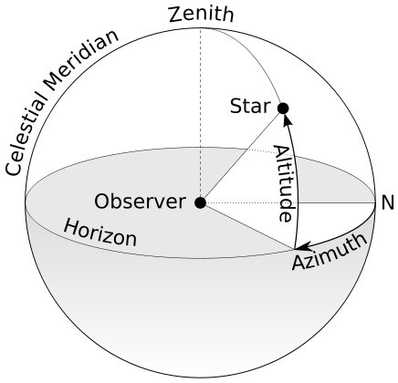
As shown in , the altitude and azimuth are defined as angles relating the direction of the star to the horizon and the north direction.
If the topocentric equatorial "of date" coordinates of an object $(X',Y',Z')$ are known, the altitude and azimuth can be computed as follows. First, compute the topocentric right ascension $\alpha$ and declination $\delta$ by $\alpha = {\rm arg}(X' + i Y')$ and $\delta = \sin^{-1}(Z'/R')$, where $R'=\sqrt{X'^2+Y'^2+Z'^2}$. Next, calculate the hour angle, $H$, by $H=t_s-\alpha$. Here $t_s$ is the local apparent sidereal time LAST. Finally, $a$ and $A$ are related to $H$ and $\delta$ by
\begin{align} \cos a \sin A &= -\cos \delta \sin H \label{eq:aAFromHdel1} \\ \cos a \cos A &= \sin \delta \cos \phi - \cos \delta \cos H \sin \phi \label{eq:aAFromHdel2} \\ \sin a &= \sin \delta \sin \phi + \cos \delta \cos H \cos \phi . \label{eq:aAFromHdel3} \end{align}The altitude computed by these formulae does not include atmospheric refraction, which is significant especially for objects close to the horizon.
Atmospheric refraction changes the altitude of an object. The effect is particularly significant for objects close to the horizon. At the horizon, refraction can raise the altitude of an object by 34'. Atmospheric refraction depends on the local temperature, pressure, humidity and other conditions. Sophisticated atmospheric refraction models involve numerical integration, but the accuracy depends on the local conditions. On the local star chart webpage, I use a low-precision fitting formula to model the atmospheric refraction. Sæmundsson's formula is used in which the change in altitude $\Delta a$ is given by
$$ \Delta a = 1.02' \left(\frac{P}{101 {\rm kPa}}\right) \left( \frac{283 {\rm K}}{T}\right) \cot \left(a + \frac{10.3^\circ}{a + 5.11^\circ}\right) , \label{eq:atmRefraction} $$where $T$ is temperature and $P$ is pressure. In all calculations, I use $T=286$ K and $P=101 {\rm kPa}$.
Given the positions of celestial objects in spherical coordinates (altitude, azimuth or GCRS Ra and Dec), the final step is to plot them on the computer screen, which is a two-dimensional flat surface. There are various methods to map a spherical surface to a flat surface. Distortion is unavoidable. Two projection methods are used in our star charts. Stereographic projection is used to generate the local star charts and the polar GCRS charts. Mollweide projection is used to generate the all-sky GCRS chart.
Stereographic projection is commonly used in sky maps. The mapping is conformal and shapes are preserved over a small area. However, the mapping does not preserve area. For example, in the local star charts a constellation is about twice as big when it is near the horizon than when it is near the zenith. This effect is quite noticeable in animations showing the diurnal motion of the sky. This feature might not be as bad, since constellations do appear bigger when they are close to the horizon because of the Moon illusion. However, it should be noted that stereographic projection is not designed to model the Moon illusion and so the distortion should not be regarded as a faithful representation of human perception.
Mollweide projection preserves areas but not angles. There is significant distortion in shapes in regions far away from the equator.
The local star charts are based on the horizontal coordinate system. The coordinates are $(a,A)$ (altitude and azimuth). The mapping from $(a,A)$ to the 2D flat surface $(x_g,y_g)$ is done by the stereographic projection with the nadir as the projection point. Only objects above or on the horizon ($a \geq 0$) are plotted.
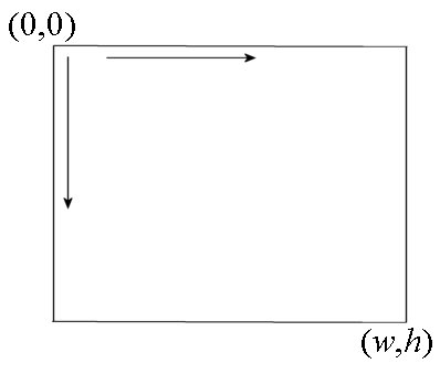
Before describing the equation of the mapping, it is useful to understand how the graph coordinate system is oriented. Graphs are drawn using the HTML canvas. As shown in , in the HTML canvas coordinates $(x_g,y_g)$ the upper-left corner is the origin $(x_g,y_g)=(0,0)$. The $x$ coordinate increases to the right and $y$ coordinates increases downward. The coordinate of the lower-right corner is $(x_g,y_g)=(w,h)$, where $w$ is the width and $h$ is the height of the canvas in pixels. In the local star charts, I set $w=h=800$ pixels.
The mapping $(a,A) \rightarrow (x_g,y_g)$ is given by
$$ r = r_h \tan\left( \frac{\pi}{4} -\frac{a}{2}\right) \ \ , \ \ x_g = \frac{w}{2} - r \sin A \ \ , \ \ y_g = \frac{h}{2} - r \cos A , \label{eq:stereographicHor} $$where $r_h = 0.47\max(w,h)$. The equation can be considered as two transformations: $a \rightarrow r$ and $(r,A) \rightarrow (x_g, y_g)$. Under this mapping, the zenith is mapped to the center of the canvas. Contours of $a$ are circles of radius $r_h\tan(\pi/4 - a/2)$ centered at the center of the canvas. Thus, the value of $r_h$ is the radius of the horizon. The value 0.47 is to make rooms for drawing labels outside the horizon.
The first chart is centered at the GCRS north pole. It is generated by the stereographic projection with the GCRS south pole as the projection point. Only the region in the northern hemisphere is shown. The third chart is centered at the GCRS south pole. It is generated by the stereographic projection with the GCRS north pole as the projection point.
In general, if $\alpha_c$ and $\delta_c$ are the GCRS right ascension and declination at the center of the chart. The mapping $(\alpha,\delta) \rightarrow (x_g,y_g)$ is given by
\begin{align} x_g &= \frac{w}{2} + \frac{r_h (\cos \delta_c \sin \delta - \sin \delta_c \cos \delta \cos \Delta \alpha )}{1 + \sin \delta_c \sin \delta + \cos \delta_c \cos \delta \cos \Delta \alpha} , \label{eq:stereographicXg} \\ \nonumber \cr y_g &= \frac{h}{2} - \frac{r_h \cos \delta \sin \Delta \alpha}{1 + \sin \delta_c \sin \delta + \cos \delta_c \cos \delta \cos \Delta \alpha} , \label{eq:stereographicYg} \end{align}where $r_h = 0.465\max(w,h)$ and $\Delta \alpha = \alpha - \alpha_c$. The width and height are set to $w=h=700$ pixels. For the first chart, $\delta_c=\pi/2$. For the third chart, $\delta_c=-\pi/2$. The value of $\alpha_c$ determines the orientation of the GCRS Ra lines. For example, if $\alpha_c=0$ in the first chart, the line $\alpha=0$ is a horizontal line from the graph center $(w/2,h/2)$ to the middle left point $(w/2 - r_h, h/2)$.
Note that when $\delta_c=\pi/2$, $\delta = a$ and $\Delta \alpha = \pi/2 - A$, equations \eqref{eq:stereographicXg} and \eqref{eq:stereographicYg} reduce to equation \eqref{eq:stereographicHor} since it can be shown that $\tan(\pi/4 - a/2) = \cos a/(1+\sin a)$.
The second GCRS chart is an all-sky chart. The GCRS right ascension at the center is set by the parameter $\alpha_c$. The canvas width and height are $w=800$ pixels and $h=400$ pixels. The chart is generated by the Mollweide projection. The mapping $(\alpha, \delta) \rightarrow (x_g,y_g)$ is given by
$$ x_g = \frac{w}{2} - r_h P\left( \frac{\alpha-\alpha_c}{\pi}\right) \cos \theta \ \ , \ \ y_g = \frac{h}{2} - \frac{r_h}{2} \sin \theta , \label{eq:mollweide} $$where $r_h = 0.465\max(w,h)$ and $\theta$ satisfies the equation
$$ 2\theta + \sin 2\theta = \pi \sin \delta .$$The above equation is solved by the Newton-Raphson method. The Newton-Raphson method usually converges to machine roundoff precision within 6 iterations. However, it may fail very close to the poles ($|\delta|\approx \pi/2$). When the Newton solver fails to converge after 20 iterations, the method of bisection is used instead, but this rarely, if ever, occurs.
In equation \eqref{eq:mollweide}, the function $P$ is defined as
$$ P(x) = x - 2 \cdot {\rm int}\left( \frac{x+1}{2} \right) $$so that $P(x) \in [-1,1)$ for any $x\in (-\infty, \infty)$ (the function int(y) returns the greatest integer smaller than or equal to y). This means that $x_g \in [w/2 - r_h, w/2 + r_h)$ and all points are inside an ellipse centered at $(w/2,h/2)$ with a semi-major axis of $r_h$ and a semi-minor axis of $r_h/2$.
In some cases (e.g. drawing constellation lines), I want to join two points $\boldsymbol{r_{g1}}=(x_{g1},y_{g1})$ and $\boldsymbol{r_{g2}}=(x_{g2},y_{g2})$ by a straight line on canvas. This is straightforward in most cases. However, in the stereographic charts, only half of the celestial sphere is plotted. If both points are inside the chart, a straight line is drawn without any problem. If both points are outside the chart, no line will be drawn (even though it is possible to have a portion of the line inside the chart). The problem arises if one of the points is outside the chart. In this case, only the part of the line inside the chart should be drawn. In the Mollweide chart, the whole celestial sphere is covered. However, in some cases it happens that the straight line connecting the two points crosses the left and right boundary of the chart. In this case, the line should be broken into two: one joining $\boldsymbol{r_{g1}}$ to the boundary and another joining $\boldsymbol{r_{g2}}$ to the boundary on the other side.
In the following I describe the mathematical detail in handling these cases.
A point $\boldsymbol{r_g}$ is inside the chart if $|\boldsymbol{r_g}-\boldsymbol{r_c}| \leq r_h$, where $\boldsymbol{r_c}=(w/2,h/2)$ is the position vector of the canvas center. Let $\boldsymbol{\xi}=\boldsymbol{r_g}-\boldsymbol{r_c}$. Also denote $\boldsymbol{\xi_1}=\boldsymbol{r_{g1}}-\boldsymbol{r_c}$ and $\boldsymbol{\xi_2}=\boldsymbol{r_{g2}}-\boldsymbol{r_c}$. Suppose that one of the two points is outside the chart. Then either $|\boldsymbol{\xi_1}| \gt r_h$ or $|\boldsymbol{\xi_2}| \gt r_h$. I will then replace the point outside the chart by a point on the line and on the chart boundary. Points on the straight line joining $\boldsymbol{r_{g1}}$ and $\boldsymbol{r_{g2}}$ can be described by the parametric equation
$$ \boldsymbol{\xi}(s) = \boldsymbol{\xi_1} + s(\boldsymbol{\xi_2}-\boldsymbol{\xi_1}) , $$where $s \in [0,1]$. The goal is to find $s$ so that $|\boldsymbol{\xi}(s)|=r_h$, which is a quadratic equation in $s$. The solution of the quadratic equation is given by
$$ s_{\pm} = \frac{\xi_1^2 - \boldsymbol{\xi_1}\cdot \boldsymbol{\xi_2} \pm \sqrt{(\xi_1^2 - \boldsymbol{\xi_1}\cdot \boldsymbol{\xi_2})^2 + (r_h^2-\xi_1^2) |\boldsymbol{\xi_2}-\boldsymbol{\xi_1}|^2}} {|\boldsymbol{\xi_2}-\boldsymbol{\xi_1}|^2} . $$The solution $s=s_+$ should be used if $|\boldsymbol{\xi_2}| \gt r_h$ and $s=s_-$ should be used if $|\boldsymbol{\xi_1}| \gt r_h$.
In summary, if $\boldsymbol{r_{g2}}$ is outside the chart, the straight line should be the line joining $\boldsymbol{r_{g1}}$ to $\boldsymbol{r_{g3}}$, where
$$ \boldsymbol{r_{g3}} = \boldsymbol{r_{g1}} + s_+ (\boldsymbol{r_{g2}}-\boldsymbol{r_{g1}}) . $$If $\boldsymbol{r_{g1}}$ is outside the chart, the straight line should be the line joining $\boldsymbol{r_{g2}}$ to $\boldsymbol{r_{g3}}$, where
$$ \boldsymbol{r_{g3}} = \boldsymbol{r_{g1}} + s_- (\boldsymbol{r_{g2}}-\boldsymbol{r_{g1}}) . $$The central GCRS Ra is specified by the parameter $\alpha_c$. The left and right boundary of the chart is $\alpha=\alpha_c +\pi$. Given two points $\boldsymbol{r_{g1}}$ and $\boldsymbol{r_{g2}}$, first determine whether the line joining them crosses the boundary by calculating the following three quantities
$$ \Delta x_1 = P \left(\frac{\alpha_1-\alpha_c-\pi}{\pi}\right) \ \ , \ \ \Delta x_2 = P\left(\frac{\alpha_2-\alpha_c-\pi}{\pi}\right) \ \ , \ \ \Delta x_{12} = P\left(\frac{\alpha_1-\alpha_2}{\pi}\right) . $$The line will cross the boundary if the following conditions are satisfied: (1) $\Delta x_1 \Delta x_2 \lt 0$ and (2) $|\Delta x_1| + |\Delta x_2| = |\Delta x_{12}|$. The first condition says that $\alpha_1$ and $\alpha_2$ are on the opposite side of the boundary Ra. The second condition says that the line that crosses the Ra boundary is the shortest line joining the two points. As an example, suppose $\boldsymbol{r_{g1}}=(-\pi/4,\delta_1)$, $\boldsymbol{r_{g2}}=(\pi/2,\delta_2)$ and $\alpha_c=0$. It follows that $\Delta x_1 = 3/4$, $\Delta x_2=-1/2$ and $\Delta x_{12}=-3/4$. It is clear that $\alpha_1$ and $\alpha_2$ are on opposite sides of the boundary Ra $\alpha_b=\pi$, but the shortest line joining the two point passes through $\alpha=0$ instead of $\alpha=\pi$ and so the line does not cross the boundary Ra. The second condition is violated in this case. Suppose that $\alpha_c=\pi$. Then the boundary Ra is $\alpha_b=0$ and so the line crosses the boundary. In this case, $\Delta x_1=-1/4$, $\Delta x_2=1/2$, $\Delta x_{12}=-3/4$, and both conditions are indeed satisfied.
Suppose that the shortest line joining the two points does cross the boundary Ra. The line will be split into two: a line joining $\boldsymbol{r_{g1}}$ and $\boldsymbol{r_{g3}}$, and a line joining $\boldsymbol{r_{g2}}$ and $\boldsymbol{r_{g4}}$, where $\boldsymbol{r_{g3}}$ is on the chart boundary closest to $\boldsymbol{r_{g1}}$ and $\boldsymbol{r_{g4}}$ is on the chart boundary closest to $\boldsymbol{r_{g2}}$.
To calculate $\boldsymbol{r_{g3}}$, first compute the following vectors
$$ \boldsymbol{\xi_1} = \frac{\boldsymbol{r_{g1}}-\boldsymbol{r_c}}{r_h} \ \ , \ \ \boldsymbol{\xi_2} = \frac{\boldsymbol{r_{g2}}-\boldsymbol{r_c}}{r_h} . $$Next compute $\boldsymbol{\xi'_2} = (\xi'_{2x} , \xi_{2y})$, where
$$ \xi'_{2x} = \left \{ \begin{array}{ll} \xi_{2x} + 2\cos \theta_2 & {\rm if}\ x_1 \gt 0\ \\ \xi_{2x} -2\cos \theta_2 & {\rm if}\ x_1 \lt 0\ \end{array} \right. , \label{eq:xip2x} $$and $\theta_2$ satisfies the equation $2\theta_2 + \sin 2\theta_2 = \pi \sin \delta_2$.
Defined in this way, the point $\boldsymbol{r'_{g2}}=\boldsymbol{x_c}+r_h \boldsymbol{\xi'_2}$ is outside the chart. Next find $\boldsymbol{r_{g3}}$ on the line joining $\boldsymbol{r_{g1}}$ and $\boldsymbol{r'_{g2}}$ and on the chart boundary. Points on the line joining $\boldsymbol{r_{g1}}$ and $\boldsymbol{r'_{g2}}$ can be parameterized by the equation
$$ \boldsymbol{\xi}(s) = \boldsymbol{\xi_1} + s(\boldsymbol{\xi'_2} - \boldsymbol{\xi_1}) , $$where $s \in [0,1]$. The boundary of the chart is an ellipse centered at $\boldsymbol{r_c}$ with a semi-major axis $r_h$ and a semi-minor axis $r_h/2$. Hence, the point $\boldsymbol{\xi}$ is on the boundary if $\xi_x^2 + 4\xi_y^2=1$, which is a quadratic equation in $s$. The solution is given by
$$ s = \frac{1-\xi_{1x}^2 - 4\xi_{1y}^2}{\xi_{1x}\Delta \xi_x + 4\xi_{1y} \Delta \xi_y + \sqrt{(\xi_{1x}\Delta \xi_x + 4\xi_{1y}\Delta \xi_y)^2 + (\Delta \xi_x^2 + 4\Delta \xi_y^2)(1-\xi_{1x}^2 - 4\xi_{1y}^2)}} , $$ $$ \Delta \xi_x = \xi'_{2x}-\xi_{1x} \ \ , \ \ \Delta \xi_y = \xi_{2y} - \xi_{1y} , \nonumber $$and $\boldsymbol{r_{g3}}$ is given by
$$ \boldsymbol{r_{g3}} = \boldsymbol{r_c} + r_h[\boldsymbol{\xi_1} + s(\boldsymbol{\xi'_2}-\boldsymbol{\xi_1})] = \boldsymbol{r_{g1}} + r_h s (\boldsymbol{\xi'_2}-\boldsymbol{\xi_1}) . $$Having computed $\boldsymbol{r_{g3}}=(x_{g3},y_{g3})$, $\boldsymbol{r_{g4}}=(x_{g4},y_{g4})$ can be computed by the equation
$$ x_{g4} = \frac{w}{2}-x_{g3} \ \ , \ \ y_{g4} = y_{g3} .$$Ecliptic is plotted on a local star chart when the Ecliptic button below the chart is active. Ecliptic is plotted on the GCRS charts when the Ecliptic button on the GCRS page is active. Galactic equator is plotted on a local star chart when the Galactic button below the chart is active. Galactic equator is plotted on the GCRS charts when the Galactic button on the GCRS page is active.
In this section, I discuss the mathematical detail in plotting the equator, ecliptic and galactic equator, which are all great circles on the celestial sphere. They can be defined as the plane perpendicular to a pole. The general strategy is first to calculate the position of the pole in the coordinate system the chart is based on. Then the coordinates of points on the great circle perpendicular to the pole can be parameterized by a parameter θ.
The coordinate system the local star charts based on is the horizontal coordinate system. First calculate the altitude $a_p$ and azimuth $A_p$ of the pole. Either a north pole or a south pole will work. I choose the north pole.
The "of date" declination of the celestial north pole is $\delta=\pi/2$. The "of date" Ra and Dec of the ecliptic north pole are $\alpha_p=-\pi/2$ and $\delta_p = \pi/2-\epsilon_A$, where the mean obliquity of the ecliptic of date is computed by equation (10) and Table 3 in Vondrák, Capitaine and Wallace. The Ra and Dec of the galactic north pole with respect to J2000.0 mean equator and equinox are $\alpha_{p0} = 12^{\rm h} 51^{\rm m} 26^{\rm s}$ and $\delta_{p0} = 27^\circ 07' 42''$. The "of date" mean equatorial coordinates at other times are computed by applying the precession matrix on the J2000.0 coordinates. Specifically, the vector $\boldsymbol{X_p}=\boldsymbol{P_0}(T) \boldsymbol{X_{p0}}$ is calculated, where $\boldsymbol{X_{p0}}$ is a column vector defined as
$$ \boldsymbol{X_{p0}}=(\cos \alpha_{p0} \cos \delta_{p0}\ \sin \alpha_{p0} \cos \delta_{p0} \ \sin \delta_{p0})^T $$and the precession matrix $\boldsymbol{P_0}(T)$ is calculated by equations (20), (11), (13), Tables 4, 6 in Vondrák, Capitaine and Wallace. The "of date" Ra and Dec of the galactic north pole is then given by $\alpha_p = {\rm arg}(X_p+iY_p)$ and $\delta_p = \sin^{-1} Z_p$. Note that $|\boldsymbol{X_p}|=|\boldsymbol{X_{p0}}|=1$ by construction.
Having computed the "of date" mean equatorial position of the pole, the hour angle is calculated approximately by $H_p=t_s - \alpha_p$, where $t_s$ is the local apparent sidereal time (LAST) computed by $t_s = {\rm GAST}+\lambda$. Here $\lambda$ is the longitude of the location and GAST is computed by equations \eqref{def:UT1} and \eqref{eq:GAST}.
The altitude $a_p$ and azimuth $A_p$ are obtained by equations \eqref{eq:aAFromHdel1}-\eqref{eq:aAFromHdel3}. Next calculate a vector $\boldsymbol{r_p} = (\cos A_p \cos a_p, \sin A_p \cos a_p, \sin a_p)$, which is a unit vector pointing in the direction of the pole in the horizontal coordinate system. Denote $\boldsymbol{r_z}=(0,0,1)$ the unit vector pointing towards the zenith. Define two unit vectors $\boldsymbol{V}$ and $\boldsymbol{W}$ as follows:
$$ \boldsymbol{V} = \frac{\boldsymbol{r_z}\times \boldsymbol{r_p}}{|\boldsymbol{r_z}\times \boldsymbol{r_p}|} \ \ , \ \ \boldsymbol{W} = \boldsymbol{r_p} \times \boldsymbol{V} . $$It follows that both $\boldsymbol{V}$ and $\boldsymbol{W}$ are perpendicular to $\boldsymbol{r_p}$ and so are on the great circle of interest. The great circle can be parameterized by the unit vector
$$ \boldsymbol{C}(\theta) = \cos \theta \, \boldsymbol{V} + \sin \theta \, \boldsymbol{W} , $$where $\theta \in [0,2\pi)$. The altitude and azimuth associated with $\boldsymbol{C}(\theta)$ are $A(\theta)={\rm arg}(C_x(\theta) + i C_y(\theta))$ and $a(\theta) = \sin^{-1} C_z(\theta)$. The set of points $\{ a(\theta), A(\theta) \}$, $\theta \in [0,2\pi)$ represents the great cicle in the horizontal coordinate system. In addition, it is easy to show that
$$ \boldsymbol{r_z} \cdot \boldsymbol{C}(\theta) = \frac{1-(\boldsymbol{r_z}\cdot \boldsymbol{r_p})^2} {|\boldsymbol{r_z}\times \boldsymbol{r_p}|} \sin \theta .$$It follows that $\boldsymbol{r_z} \cdot \boldsymbol{C}(\theta) \geq 0$ for $\theta \in [0,\pi]$. These are the points on the great circle that are above or on the horizon. The canvas coordinates of these points are calculated by equation \eqref{eq:stereographicHor}. These points can then be joined by a curve representing the great circle on the canvas.
The coordinate system is the GCRS equatorial coordinate system, which is essentially the same as the J2000.0 mean equatorial coordinate system except for the 17-milliarcsecond offset between their poles. I treat these two systems as identical because of the small offset. In this coordinate system, the coordinates of the north pole of the ecliptic of date are $\alpha_p = \gamma-\pi/2$ and $\delta_p = \pi/2 - \varphi$. The angles $\gamma$ and $\varphi$ are calculated from equation (14) and Table 7 in Vondrák, Capitaine and Wallace. The coordinates of the galactic north pole are $\alpha_{p} = 12^{\rm h} 51^{\rm m} 26^{\rm s}$ and $\delta_{p} = 27^\circ 07' 42''$.
The procedure of plotting the great circle perpendicular to the pole is similar to that described in the previous subsection. The unit vector associated with the pole is computed by $\boldsymbol{r_p} = (\cos \alpha_p \cos \delta_p, \sin \alpha_p \cos \delta_p, \sin \delta_p)$. The unit vector associated with the GCRS north pole is $\boldsymbol{r_z}=(0,0,1)$. Define two unit vectors
$$ \boldsymbol{V} = \frac{\boldsymbol{r_z}\times \boldsymbol{r_p}}{|\boldsymbol{r_z}\times \boldsymbol{r_p}|} \ \ , \ \ \boldsymbol{W} = \boldsymbol{r_p} \times \boldsymbol{V} . $$It follows that both $\boldsymbol{V}$ and $\boldsymbol{W}$ are perpendicular to $\boldsymbol{r_p}$ and so are on the great circle of interest. The great circle can now be parameterized by the unit vector
$$ \boldsymbol{C}(\theta) = \cos \theta \, \boldsymbol{V} + \sin \theta \, \boldsymbol{W} , $$where $\theta \in [0,2\pi)$. The GCRS Ra and Dec associated with $\boldsymbol{C}(\theta)$ are $\alpha(\theta) = {\rm arg}(C_x(\theta) + i C_y(\theta))$ and $\delta(\theta) = \sin^{-1} C_z(\theta)$. The set of points $\{ \alpha(\theta), \delta(\theta) \}$, $\theta \in [0,2\pi)$ represents the great cicle in the GCRS coordinate system. The canvas coordinates of these points are given by equations \eqref{eq:stereographicXg}-\eqref{eq:stereographicYg} for the polar charts and equation \eqref{eq:mollweide} for the all-sky chart. Half of the great circle will appear on each of the polar charts and the full great circle will appear in the all-sky chart.
The star data used on our webpages are a subset of the HYG 3.0 database. The database is constructed using the following procedure. All data processing was done using the R software.
- Remove the Sun, Capella B and α Cen B from the database. Capella B and Capella A are too close to be separated on our star charts. They have slightly different 3D motions (constructed from the database) that will separate them in the distant future and distant past. That is why Capella B is removed. α Cen B is removed for the same reason.
- The ICRS rectangular coordinates of each star are computed from their distance $D_0$, J2000.0 $\alpha_0$ and $\delta_0$ by $x_0=D_0 \cos \alpha_0 \cos \delta_0$, $y_0=D_0\sin \alpha_0 \cos \delta_0$ and $z_0=D_0 \sin \delta_0$. These are components of the ICRS position vector $\boldsymbol{r(t)}$ at $t=$J2000.0. Note that a value of 100,000 is assigned to $D_0$ if the distance of a star is unknown or its value is dubious. This will not cause much trouble since it is the angular direction of the star that is important, but it needs to be kept in mind for calculations involving $D_0$.
- ICRS components of a star's 3D velocity is computed from its distance $D_0$, J2000.0 $\alpha_0$ and $\delta_0$, proper motions $\mu_{\alpha}$, $\mu_{\delta}$ and radial velocity $v_r$ according to the equation \begin{align} \boldsymbol{v} &= D_0 \mu_{\alpha} \boldsymbol{e_{\alpha}} + D_0\mu_{\delta} \boldsymbol{e_{\delta}} + v_r \boldsymbol{e_r} , \\ \boldsymbol{e_{\alpha}} &= -\sin \alpha_0 \cos \delta_0 \boldsymbol{\hat{x}} + \cos \alpha_0 \cos \delta_0\boldsymbol{\hat{y}} \\ \boldsymbol{e_{\delta}} &= -\cos \alpha_0 \sin \delta_0 \boldsymbol{\hat{x}} -\sin \alpha_0 \sin \delta_0 \boldsymbol{\hat{y}} + \cos \delta_0 \boldsymbol{\hat{z}} \\ \boldsymbol{e_r} &= \cos \alpha_0 \cos \delta_0 \boldsymbol{\hat{x}} + \sin \alpha_0 \cos \delta_0 \boldsymbol{\hat{y}} + \sin \delta_0 \boldsymbol{\hat{z}} . \end{align} All components of $\boldsymbol{v}$, $v_x$, $v_y$ and $v_z$, are converted to pc/(Julian century) for convenience of later calculations.
- Our webpages draw star charts in the time range J2000.0±200,000 years. For stars with reliable measured distance ($D_0 \neq 10^5$), their minimum distance and magnitude in the time intervals J2000.0±200,000 years are calculated as follows. The ICRS position vector of the star as a function of t (neglecting light-time correction) is given by $$ \boldsymbol{r}(t) = \boldsymbol{r_0} + \boldsymbol{v} \Delta t , $$ where $\boldsymbol{r_0}$ is the position vector of the star at $t=t_0$=J2000.0 and $\Delta t = t-t_0$. Here it is assumed that the star moves with a constant velocity $\boldsymbol{v}$. The distance is minimum when $\boldsymbol{v}\cdot \boldsymbol{r}(t)=0$, which gives $$ \Delta t_{\rm min} = -\frac{\boldsymbol{r_0}\cdot \boldsymbol{v}}{v^2} . $$ Since time is restricted to $|\Delta t| \lt 2\times 10^5$ years, set $\Delta t_{\rm min} =-2\times 10^5$ years if $\Delta t_{\rm min} \lt -2\times 10^5$ years and $\Delta t_{\rm min} =2\times 10^5$ years if $\Delta t_{\rm min} \gt 2\times 10^5$ years. Then the minimum distance in the time interval is $$ D_{\rm min} = |\boldsymbol{r_0} + \boldsymbol{v} \Delta t_{\rm min}| $$ and the minimum magnitude of the star is calculated by the inverse square law as $$ m_{\rm min} = m_0 + 5 \log_{10} (D_{\rm min}/D_0) , $$ where $m_0$ is the star's magnitude at $t=t_0$ and $D_0=|\boldsymbol{r_0}|$ is the star's distance at $t=t_0$.
- Stars with $m_{\rm min} \gt 5.3$ are removed from the database since 5.3 is the limiting magnitude of stars that will be plotted on our star charts. The resulting database contains 2559 stars.
- For the purpose of drawing constellation lines, certain stars are manually selected for each constellation line segment. They are specified by either the star's proper name, Bayer/Flamsteed name, or hip number. They are then converted to the index numbers in the database.
- For each of the 88 constellations, approximate values of the ICRS Ra and Dec of the constellation are entered manually. The constellation labels, when active, will be plotted at these locations. For the constellations Hydra, Serpens and Eridanus, two locations are indicated because of their large size or topology.
- The final data are put into JSON format and outputted to the JavaScript file
brghtStars.js, which contains functions returning JavaScript objects.
Light-time correction arises from the finite speed of light. It is usually included in the calculation of the apparent positions of planets, but usually not applied to the positions of stars because their motion and distance are not known accurately. Our webpages do not include light-time correction for stars. The detail calculation is presented here so that it can be implemented when accurate data are available in the future. The equations derived in this subsection are essentially the same as those in Stumpff [A&A 144, 232 (1985)], but are derived using a different approach.
The observed barycentric position of a star at time $t$ is the "true" position of the star at the retarded time $t_r$
$$ \boldsymbol{r^*}(t) = \boldsymbol{r}(t_r) . \label{def:rstar} $$The retarded time $t_r$ satisfies the equation
$$ t_r(t) = t - \frac{D(t_r)}{c} , \label{eq:tr} $$where $D(t_r) = |\boldsymbol{r}(t_r)|$ is the barycentric distance of the star at the retarded time and $c$ is the speed of light. Differentiating equation \eqref{def:rstar} with respect to $t$ gives
$$ \boldsymbol{v^*}(t) = \boldsymbol{\dot{r}^*}(t) = \boldsymbol{v}(t_r) \frac{d t_r}{dt} . \label{eq:vstar1} $$It follows from \eqref{eq:tr} that
$$ \frac{dt_r}{dt} = 1-\frac{v_r}{c} \frac{dt_r}{dt} \ \ \ \Rightarrow \ \ \ \frac{dt_r}{dt} = \frac{1}{1+\beta_r(t_r)} , \label{eq:dtr_dt} $$where $v_r = d D/dt$ is the radial velocity and $\beta_r = v_r/c$. Combining equations \eqref{eq:vstar1} and \eqref{eq:dtr_dt} gives
$$ \boldsymbol{v^*}(t) = \frac{\boldsymbol{v}(t_r)}{1+\beta_r(t_r)} .$$Thus, the observed tangential velocity, $\boldsymbol{v^*}_T(t)=D\mu_{\alpha}\boldsymbol{e_{\alpha}} + D \mu_{\delta} \boldsymbol{e_{\delta}}$ is related to the true tangential velocoty at the retarded time $\boldsymbol{v}_T(t_r)$ by
$$ \boldsymbol{v^*}_T(t) = \frac{\boldsymbol{v}_T(t_r)}{1+\beta_r(t_r)} . \label{eq:vTstar} $$This formula explains the origin of the observed superluminal motion of jets in some active galaxies: if a jet moving close to the speed of light is moving at a very small angle towards the observer, $1+\beta_r \ll 1$ and it is possible to have $v^*_T \gt c$. Equation \eqref{eq:vTstar} is usually derived by drawing a figure showing the geometry between the source and observer. The derivation presented here is mathematically more straightforward but the physics behind the formula is illustrated more clearly in the conventional derivation. For stars in the vicinity of the Sun, $\beta_r \sim 10^{-4}$ and so the correction to the tangential velocity is very small. The radial velocity $v_r$ is related to the redshift $z$ by the special relativistic Doppler formula
$$ 1 + z = \frac{1+\beta_r}{\sqrt{1-\beta^2}} , \label{eq:z} $$where $\beta = v/c = \sqrt{v_T^2+v_r^2}/c$. Thus, equations \eqref{eq:vTstar} and \eqref{eq:z} must be solved together to obtain $\boldsymbol{v}_T$ and $v_r$ from the observed quantities $\boldsymbol{v^*}_T$ and $z$. Once $\boldsymbol{v}_T$ and $v_r$ are computed, the true velocity $\boldsymbol{v}(t_r)$ is obtained. I assume that $\boldsymbol{v}$ is constant, which is in general a good approximation since the time scale of galactic rotation in the solar neighborhood is $10^8$ years and is much longer than the time span considered here.
Suppose the apparent position at time $t_0$, $\boldsymbol{r^*}(t_0)$, and the velocity $\boldsymbol{v}$ is known, the observed position at time $t=t_0+\Delta t$ is given by
$$ \boldsymbol{r^*}(t) = \boldsymbol{r}(t_r(t)) \label{eq:rstar1} $$with
\begin{align} t_r(t) &= t - \frac{D(t_r(t))}{c} = t_0 + \Delta t - \frac{D(t_r(t_0))}{c} + \frac{D(t_r(t_0)) - D(t_r(t))}{c} \nonumber \cr \nonumber \cr &= t_r(t_0) + (1+f) \Delta t , \label{eq:tr2} \end{align}where
$$ f = \frac{D(t_r(t_0))-D(t_r(t))}{c \Delta t} . \label{eq:f1} $$Denote $\boldsymbol{r^*_0} = \boldsymbol{r^*}(t_0) = \boldsymbol{r}(t_r(t_0))$, $D_0 = D(t_r(t_0)) = |\boldsymbol{r^*_0}|$, and $D=D(t_r(t))=|\boldsymbol{r^*}(t)|$. It follows from equation \eqref{eq:rstar1}, \eqref{eq:tr2} and $\boldsymbol{r}(t_2) = \boldsymbol{r}(t_1) + \boldsymbol{v}(t_2-t_1)$ that
$$ \boldsymbol{r^*}(t) = \boldsymbol{r^*_0} + (1+f)\boldsymbol{v} \Delta t . \label{eq:rstar2} $$It follows from \eqref{eq:f1} that
$$ D = D(t_r(t)) = |\boldsymbol{r^*}(t)| = D_0 - f c \Delta t . \label{eq:D} $$Combining equations \eqref{eq:rstar2} and \eqref{eq:D} yields
$$ D_0 - f c \Delta t = |\boldsymbol{r^*_0} + (1+f)\boldsymbol{v} \Delta t| .$$Squaring both sides of the above equation gives
$$ (D_0 - f c \Delta t)^2 = D_0^2 + 2(1+f)\Delta t \boldsymbol{r^*_0} \cdot \boldsymbol{v} + (1+f)^2 v^2 \Delta t^2 . $$This is a quadratic equation in $f$ and the solution is given by
$$ f = -\frac{2 \boldsymbol{s_0}\cdot \boldsymbol{\beta} + \beta^2 \Delta t}{s_0 + \boldsymbol{s_0}\cdot \boldsymbol{\beta} + \beta^2 \Delta t + \sqrt{Q}} , \label{eq:f2} $$where $\boldsymbol{s_0} = \boldsymbol{r^*_0}/c$, $\boldsymbol{\beta}=\boldsymbol{v}/c$, $s_0 = |\boldsymbol{s_0}|$, $\beta = |\boldsymbol{\beta}|$ and
$$ Q = (s_0 + \boldsymbol{s_0}\cdot \boldsymbol{\beta} + \beta^2 \Delta t)^2 + (1-\beta^2)(2\boldsymbol{s_0}\cdot \boldsymbol{\beta} + \beta^2 \Delta t) . $$Equations \eqref{eq:rstar2} and \eqref{eq:f2} can be used to update the apparent position of a star from time $t_0$ to $t$. The term $f\boldsymbol{v}\Delta t$ is an extra term arising from the light-time correction. The value of $f$ is of order β, which is $\sim 10^{-4}$ for stars in the solar neighborhood. Since the fractional accuracy of $\boldsymbol{v}$ is much larger than $10^{-4}$ in the data used by our webpages, including the light-time correction will not improve the accuracy of a star's position.
Geocentric apparent positions of stars at a given time are required to plot the stars in the GCRS star charts. Topocentric apparent positions of stars are required to plot the stars in the local star charts. Chapter 7 of Explanatory Supplement to the Astronomical Almanac provides a detailed procedure in computing the apparent positions of stars. For geocentric apparent positions, the stars' space motion, annual parallax, gravitational deflection of light by the Sun, and annual aberration of light should be included. For topocentric positions, precession, nutation, polar motion, diurnal aberration of light and atmospheric refraction should also be included.
Apart from precession and space motion, all the other effects mentioned are periodic or nonaccumulative. Annual parallax is inversely proportional to the star's distance. It is very small. The parallax of the closest stars is about 0.75". Gravitational deflection of light is only significant if the star is in a direction very close to the Sun. However, the maximum deflection angle is only 1.75". Annual aberration of light causes a shift in a star's position by 20.5" over the course of a year. The effect of nutation is about 9". The effect of diurnal aberration is smaller than 0.32". Polar motion affects a star's position by about 0.3". Atmospheric refraction can change a star's position by 34' if it is close to the horizon. On our webpages, only the space motion, precession and atmospheric refraction are included when plotting stars.
A star's ICRS position at time $t$ (neglecting light-time correction) is calculated according to the equation
$$ \boldsymbol{r}(t) = \boldsymbol{r_0} + \boldsymbol{v} (t-t_0) ,$$where $t_0=$J2000.0 and $\boldsymbol{r_0} = D_0 (\cos \alpha_0 \cos \delta_0\ \sin \alpha_0 \cos \delta_0\ \sin \delta_0)^T$ is the ICRS position vector at $t=t_0$, $\alpha_0$ and $\beta_0$ are the star's ICRS Ra and Dec at J2000.0, and $D_0=|\boldsymbol{r_0}|=\sqrt{\boldsymbol{r_0}^T \boldsymbol{r_0}}$ is the distance of the star at $t=t_0$. Since parallax is ignored, the star's GCRS position is the same as its ICRS position: $\boldsymbol{X}(t)=\boldsymbol{r}(t)$. The GCRS Ra and Dec of the star at time $t$ is therefore $\alpha = {\rm arg}(X+iY)$ and $\delta = \sin^{-1} (Z/D)$, where $D=|\boldsymbol{X}(t)|=|\boldsymbol{r}(t)|$. The magnitude of the star at time $t$ is
$$ m(t) = m_0 + 5\log_{10}(D/D_0) ,$$where $m_0$ is the star's magnitude at $t=t_0$. The star can now be plotted on the GCRS star charts: its canvas coordinates on the star charts are given by equations \eqref{eq:stereographicXg}-\eqref{eq:mollweide}. A star is represented by a filled circle with size proportional to its magnitude $m(t)$.
To plot a star on the local star charts, altitude $a$ and azimuth $A$ are required at the given location. First, the "of date" equatorial coordinates are computed by the precession matrix: $\boldsymbol{X'}(t)=\boldsymbol{P_0}(T)\boldsymbol{X}(t)$, where $T$ is the TT Julian centuries of $t$ from $t_0$. The precession matrix $\boldsymbol{P_0}(T)$ is calculated by equations (20), (11), (13), Tables 4, 6 in Vondrák, Capitaine and Wallace. The "of date" Ra and Dec of the star is $\alpha = {\rm arg}(X'+iY')$ and $\delta=\sin^{-1} (Z'/D)$. The hour angle of the star is $H=t_s-\alpha$, where $t_s$ is the local apparent sidereal time (LAST) computed by $t_s = {\rm GAST}+\lambda$. Here $\lambda$ is the longitude of the location and GAST is computed by equations \eqref{def:UT1} and \eqref{eq:GAST}. Next $a$ and $A$ are computed using equations \eqref{eq:aAFromHdel1}-\eqref{eq:aAFromHdel3}. Then the altitude is adjusted by the atmospheric refraction according to equation \eqref{eq:atmRefraction}. The star can now be plotted on a local star chart: its canvas coordinates are given by equation \eqref{eq:stereographicHor}.
Stars in the charts can be clicked and a popup box will appear. The popup box shows further information about the star: its name, constellation, apparent magnitude, distance, spectral type, color index, J2000.0 Ra and Dec, apparent position respect to the true equator and equinox of date, altitude, azimuth, rise, set and upper transit times.
If a star's proper name is available, it is displayed in the popup box together with its Bayer name (e.g. Procyon, α CMi). If both the proper name and Bayer name are not available, Flamsteed name is displayed (e.g. 50 Cas). If proper name, Bayer name and Flamsteed name are not available, the HIP number is displayed (e.g. hip 33694).
The constellation a star is in is determined by the constellation boundaries established by the Belgian astronomer Eugène Delporte in 1930 on behalf of the IAU. The boundary data are obtained from the ftp site ftp://cdsarc.u-strasbg.fr/pub/cats/VI/42. The boundaries are always along constant right ascension and declination with respect to the mean equator and equinox in 1875. The boundary data are sorted in descending order of declination in the file data.dat in the above ftp site. It is easy to use them to determine the constellation a star is in once the Ra and Dec of the star are precessed to the epoch of 1875. In the distant past and distant future, some nearby stars are seen to move far away from their present constellations. In that case, two constellations are given. The first one has "(2000)" added to it, indicating the present constellation the star is in. The second constellation has "(year number)" added to it, indicating the constellation in that particular year.
When the time is between 3000 BCE and 3000 CE, the position of a star with respect to the J2000.0 mean equator and equinox are corrected for proper motion and annual parallax. The apparent position with respect to the true equator and equinox of date are corrected for precession, nutation, and aberration of light in addition to proper motion and parallax. Outside the time interval 3000 BCE - 3000 CE, only proper motion is included in the J2000.0 position and only precession and proper motion are included in the "of date" position.
A star's annual parallax is calculated by computing the star's geocentric position $\boldsymbol{X}$ from its BCRS position $\boldsymbol{r}$ using $\boldsymbol{X}=\boldsymbol{r}-\boldsymbol{r_E}$, where $\boldsymbol{r_E}$ is Earth's barycentric position, computed using an approximate formula provided by JPL.
After parallax is included, components of a star's position vector in the rectangular equatorial coordinates of the true equator and equinox of date are computed using the precession and nutation matrix: $\boldsymbol{X'}=\boldsymbol{NPX}$. Here $\boldsymbol{P}$ is the precession matrix $\boldsymbol{P_0}(T)$ and $\boldsymbol{N}$ is nutation matrix calculated by equation \eqref{eq:nutationMatrix}.
To compute the aberration of light, $\boldsymbol{v_E}=\boldsymbol{\dot{r}_E}$ has to be calculated first. This is done by differentiating JPL's approximate formula for $\boldsymbol{r_E}$ (see the next section). The resulting $\boldsymbol{v_E}$ is expressed in the ICRS rectangular coordinate system. It is then transformed to the rectangular equatorial coordinate system of the true equator and equinox of date by applying the precession and nutation matrix $\boldsymbol{NPv_E}$. Then the direction of the star is modified by the annual aberration according to equation \eqref{eq:aberration} with $\boldsymbol{n}=\boldsymbol{X'}/|\boldsymbol{X'}|$ and $\boldsymbol{\beta} = \boldsymbol{N P v_E}/c$. The corrected $\alpha$ and $\delta$ are given by $\alpha = {\rm arg}(n'_x + i n'_y)$ and $\delta = \sin^{-1} n'_z$. These are the apparent Ra and Dec of date displayed in the popup box of stars in the GCRS charts.
For the popup box in the local star charts, I also include diurnal aberration of light by adding $\boldsymbol{NPv_E}$ to $\boldsymbol{v_{\rm spin}}$ calculated from equation \eqref{eq:vspin}. The vector $\boldsymbol{n'}$ is calculated by equation \eqref{eq:aberration} with $\boldsymbol{\beta}=(\boldsymbol{NPv_E}+\boldsymbol{v_{\rm spin}})/c$. The resulting $\alpha$ and $\delta$ derived from $\boldsymbol{n'}$ thus include both annual and diurnal aberration of light.
The computation of stellar parallax requires $\boldsymbol{r_E}$ and the computation of stellar aberration requires $\boldsymbol{v_E}$. Both vectors are calculated based on JPL's approximate formula, which is accurate only in the time interval between 3000 BCE and 3000 CE. The formulae for the nutation matrix $\boldsymbol{N}$ also become inaccurate far away from this interval. That is why nutation, stellar parallax and aberration are not computed outside this time interval even in the popup box.
In the local star charts, altitude $a$ and azimuth $A$ in the popup box are calculated in the exact same way as in the previous subsection if the time is outside the interval 3000 BCE and 3000 CE. When the time is between 3000 BCE and 3000 CE, a star's apparent Ra and Dec corrected for space motion, parallax, precession, nutation and aberration of light are used to compute $a$ and $A$. Specifically, the hour angle is computed using $H=t_s-\alpha$, where $t_s$ is the local apparent sidereal time calculated from $t_s={\rm GAST}+\lambda$. The Greenwich apparent sidereal time is calculated using equations \eqref{def:UT1} and \eqref{eq:GAST}. Next $a$ and $A$ are computed using equations \eqref{eq:aAFromHdel1}-\eqref{eq:aAFromHdel3}. Then the altitude is adjusted by the atmospheric refraction according to equation \eqref{eq:atmRefraction}.
When the Galactic button on the webpages is active, the galactic equator is shown together with the location of the galactic center if it's inside the chart. There are several different notions of galactic center, although their locations are probably indistinguishable on our low-resolution star charts. Here we represent the galactic center by the location of the compact radio source Sagittarius A*.
The calculation of the position of Sgr A* is the same as the stars. According to Reid and Brunthaler (ApJ 616, 872, 2004; doi: 10.1086/424960), the J2000 Ra and Dec of Sgr A* are $\alpha_0=17^{\rm h}45^{\rm m}40.04^{\rm s}$ and $\delta_0 = -29^{\circ}00'28.12''$. Assuming a distance of 8kpc, the 3D position is represented by
$$ \boldsymbol{r_0} = (-0.4372574538\ -6.9827518193\ -3.8794307506)^T {\rm kpc} .$$The proper motion is given by $\boldsymbol{\mu} = (-3.151 \boldsymbol{e_E} - 5.547 \boldsymbol{e_N})$ milliarcsec/year, where $\boldsymbol{e_E}=\boldsymbol{e_{\alpha}}/\cos \delta_0$ is the unit vector in the east direction and $\boldsymbol{e_N}=\boldsymbol{e_{\delta}}$ is the unit vector in the north direction. Ignoring the radial velocity, the apparent 3D velocity of Sgr A* is
$$ \boldsymbol{v} = (-1.1545\times 10^{-5}\ \ 1.1176\times 10^{-5}\ \ -1.8815\times 10^{-5})^T {\rm kpc/century} . $$Position of Sgr A* at time $T$ centuries after J2000 is given by $\boldsymbol{r}(T) = \boldsymbol{r_0} + \boldsymbol{v} T$. At the distance of 8kpc, the parallax is 0.000125" and can be ignored.
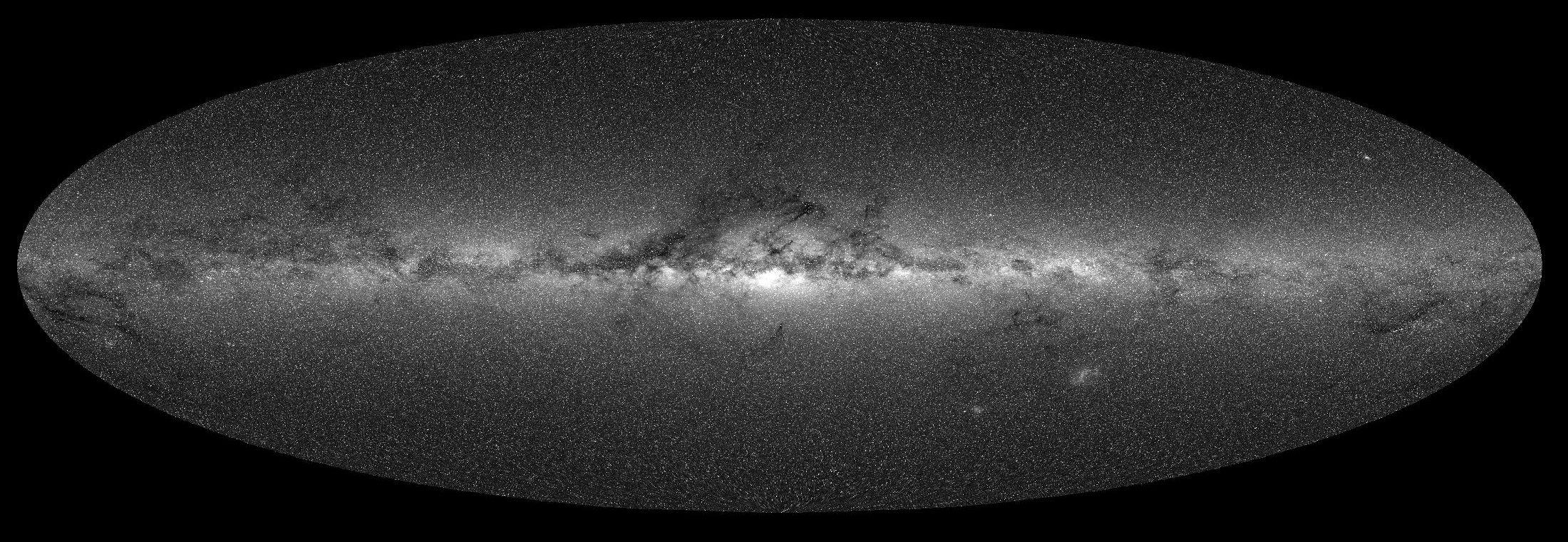
Milky Way is the hazy band of white light across the sky produced by numerous amount of stars each of which is invisible to the eye. Modern astronomical instruments are able to resolve the Milky Way into stars. Thanks to the Gaia mission, we now have accurate positions and photometric data of 1.8 billion stars from the Gaia Early Data Release 3 (EDR3). The above image is created by adding the light of 300 million brightest stars with magnitude larger than 6.5 from EDR3. When the full data are used, the resulting image is even more stunning.
The generation of the image is straightforward. Data of 300 million stars were first downloaded from the Gaia archive using the ADQL query, which is very useful in extracting a subset of the data. Only stars with magnitude larger than 6.5 were requested and the data were sorted in descending order of the G-band photometric mean flux. The 300 million data cover stars with magnitude down to 17.976336.
Next the whole sky was divided into regions of equal area. The positions of stars in the Gaia data are given in the ICRS. However, galactic coordinates are more suitable for our purpose. Hence the ICRS right ascension $\alpha$ and declination $\delta$ were tranformed to the galactic longitude $l$ and latitude $b$ using the equations
\begin{align} \sin b &= \sin \delta_{\rm NGP} \sin \delta + \cos \delta_{\rm NGP} \cos \delta \cos (\alpha - \alpha_{\rm NGP}) \nonumber \cr \cos b \sin (l_{\rm NCP} - l) &= \cos \delta \sin (\alpha - \alpha_{\rm NGP}) \\ \cos b \cos (l_{\rm NCP} - l) &= \cos \delta_{\rm NGP} \sin \delta - \sin \delta_{\rm NGP} \cos \delta \cos (\alpha - \alpha_{\rm NGP}) , \nonumber \end{align}where $\alpha_{\rm NGP}=12^{\rm h} 51.4^{\rm m}$ and $\delta_{\rm NGP}=27.13^{\circ}$ are the right ascension and declination of the galactic north pole, $l_{\rm NCP}=122.93^{\circ}$ is the galactic longitude of the north celestial pole.
Since the differential solid angle is $d\Omega = \cos b dl db = dl d(\sin b)$, an easy way to divide the whole sky into non-overlapping regions of equal area is to use constant longitude and latitude lines. In particular, the galactic longitude was divided into $n_l$ equally spaced intervals $\Delta l = 2\pi/n_l$ radians and the sine of galactic latitude was divided into $n_b$ equally spaced intervals $\Delta \sin b = 2/n_b$. Then each of the $n_l\times n_b$ region covered a solid angle
$$ \Delta \Omega = \Delta l \Delta (\sin b) = \frac{4\pi}{n_l n_b} \mbox{steradians} = \frac{129600}{\pi n_l n_b} \mbox{ square degrees} . $$The surface brightness of the sky in each region was then computed by
$$ B({\rm region}) = \frac{1}{\Delta \Omega} \sum_{{\rm star} \in{\rm region}} F_{\rm star} , $$where $F_{\rm star}$ was the photometric mean flux of the star in units of e-/s in the Gaia data. Values of $B$ may be converted to more familiar units such as cd/m2 or mag/arcsec2 but it was not necessary since I was mainly interested in the relative surface brightness in different regions.
is based on the data with $n_l=2000$ and $n_b=735$, so each region covers 0.028 square degrees, which is about 14% of the solid angle subtended by the full Moon. Since there are 300 million stars in these 2000×735=1.47 million regions, each region has on average 204 stars. However, stars are not uniformly distributed in the sky. It turns out that the number of stars in each region varies from 0 to 20837.
Note that only 300 million stars of the 1.8 billion stars in the Gaia data were used in the calculation. The main reason was to speed up computation and to avoid downloading huge amount of data. Although each dim star contributes less to the overall light, there are more of them so collectively dimmer stars contribute about the same as the brighter stars until we go dim enough to the point when we reach distances to the scale height of our Galaxy's disk and to distances at which interstellar extinction becomes significant. By comparing the results of using 180 million stars and 300 million stars, I find that although the surface brightness $B({\rm region})$ in each region has not converged, about half of the relative surface brightness
$$ \bar{B}({\rm region}) = \frac{B({\rm region})}{B_{\rm median}}$$changes by less than 1.3%. Here $B_{\rm median}$ is the median of the surface brightness in the 1.47 million regions. By comparing to the image released by ESA/Gaia/DPAC we see that most of the promonent features are present in . However, the Magellanic clouds are less promonent in compared to the release image. This is not surprising since at distances of 50kpc and 60kpc, only stars more luminous than about $135L_{\odot}$ and $200L_{\odot}$ can have apparent magnitudes smaller than 17.98, where $L_{\odot}$ is the solar luminosity. Hence the 300 million star data miss a large number of lower luminosity stars in the two galaxies.
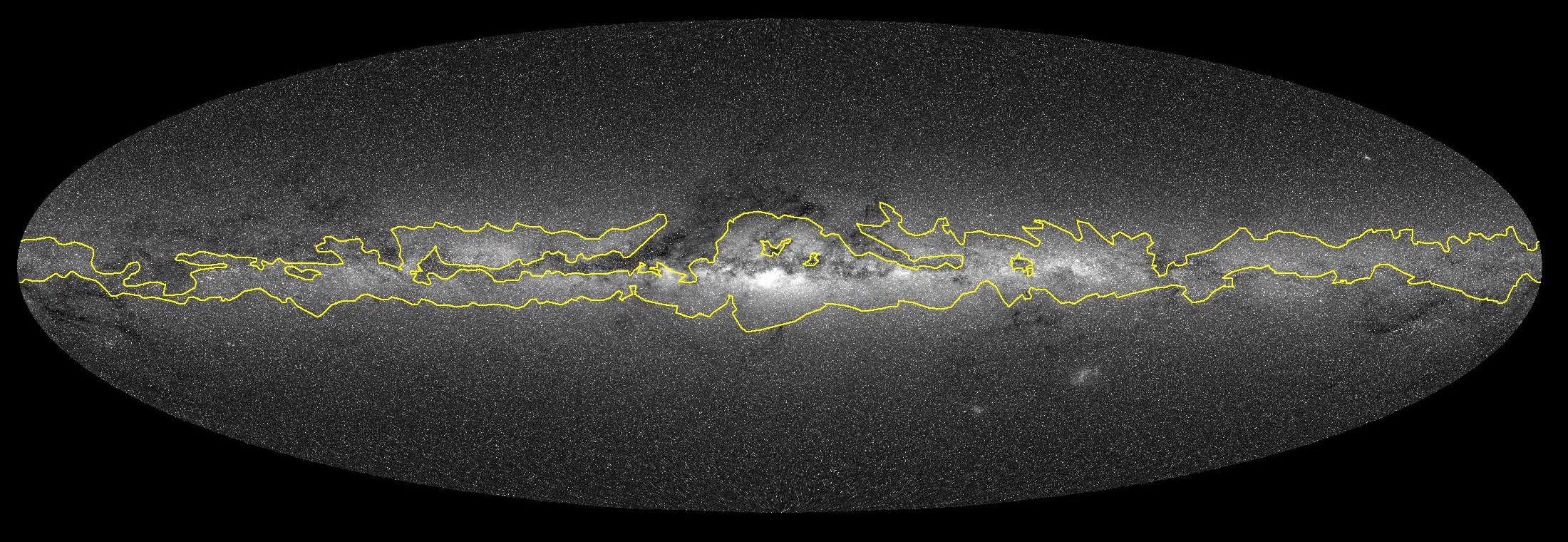
The features shown in also match photos of Milky Way. However, some features are clearly beyond naked-eye visibility. So I created a cartoon version of the picture to depict the Milky Way visible by the eye. It's based on the Milky Way boundary data provided by Jarmo Moilanen. plots this boundary (yellow line) on top of the image constructed from the Gaia data.
We can see that the approximate boundary data roughly match the simulated image. The surface brightness of the Milky Way is not uniform. The brightest regions are concentrated in galactic longitudes between about -80° and 0°, passing the constellations Carina, Crux, Centaurus, Norma, Ara, Scorpius and Sagittarius. Outside these regions, the surface brightness generally decreases with increasing galactic longitude $|l|$ and reaches minima in $155^{\circ} \lesssim l \lesssim 180^{\circ}$ (in Perseus and Auriga). The cartoon version ignores the patchy bright spots and models the Milky Way surface brightness as a function of galactic longitude. shows the cartoon version of the Milky Way used in our star charts. The relatively low contrast between the cartoon Milky Way and background is chosen to reflect the reality that the Milky Way is faint and even invisible in light polluted skies.
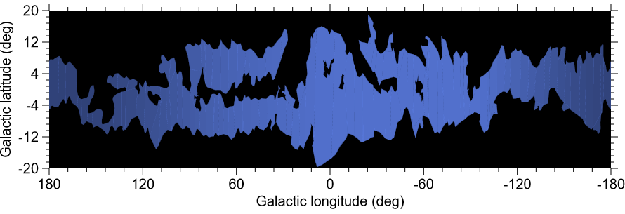
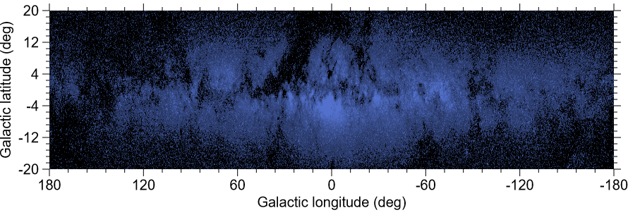
This cartoon picture is of course not ideal. shows another rendition of the Milky Way, which is generated using the Gaia data to capture the variation of surface brightness in various regions of the Milky Way more accurately. Regions with low surface brightness are removed to approximately match the boundary data. I decide not to use this version for the star chart pages because it requires more computational resource to render. In reality, Milky Way's visual appearance is sensitive to the brightness of the background sky and probably also sensitive to the acurity of one's vision. Given the amorphous appearance of the Mily Way, the cartoon picture is adequate for the relatively low-resolution star charts on our website.
The cartoon Milky Way is broken up into 125 non-overlapping regions. Each region is represented by a polygon defined by a set of vertex points. The first and last vertex points are the same, so the vertices trace out a closed loop. Each vertex is represented by the right ascension and declination with respect to the mean equator and equinox of J2000. These coordinates are then transformed to the canvas coordinates for plotting. Each polygon is also assigned a relative surface brightness between 0 and 1, which is used to set the opacity of the polygon.
Drawing the cartoon Milky Way on an HTML canvas is mostly straightforward, but there are some subtle issues. Most of the time we just need to trace the vertices of the polygons and then fill the interior region. In the star charts using the stereographic projection, some polygons will be partly or entirely outside the chart. With the canvas clip() method, polygons that are partly outside the chart can be drawn in the same way as the ones that are entirely inside. However, it's important not to draw any polygon whose vertices are all far outside the chart. This is because the projection point of a stereographic map is a singular point. If a polygon encircles the projection point, the projection will map the vertex points on opposite sides of the chart. So even though all the vertices are outside the chart, the interior of the mapped vertices will intersect the plotting area.
Drawing polygons in a Mollweide chart is a little tricky. Most of the time the polygons can be drawn in the usual way, but an issue arises when a polygon crosses the left or right boundary because it will continue on the opposite side of the boundary. We need to tell canvas what regions to fill as it doesn't know how the boundary points are identified. We will have to check whether the vertices in a polygon cross a boundary using the three conditions mentioned in Section 12.3.2. If boundary crossings occur, two branches are created: one on the left and the other on the right. Let the first branch be on the side of the vertex just before the first boundary crossing. Then the canvas coordinates of points before the first boundary crossing and after even number of crossings are in this branch. Points after odd number of boundary crossings are on the other side and need to be shifted horizontally. The shift is implemented using an equation similar to \eqref{eq:xip2x}. Points in the second branch need to be shifted horizontally before the first boundary crossing and after even number of crossings. These rules will ensure the polygons in the two branches are filled appropriately. The clip() method is also needed since the shifted points are outside the plotting area. For a general polygon, the number of boundary crossings can be none or any other even numbers. Even though the current code can handle the general case, I have not seen more than two boundary crossings in the 125 polygons. This is in large part due to the creation the polygons: the cartoon picture is carefully broken into pieces so that each piece has a relatively simple shape.
For the purpose of plotting the Sun and planets on the star charts, the heliocentric position $\boldsymbol{r}$ of each of the eight planets in the solar system is computed by the low-precision formulae provided by JPL (also given in Section 8.10 of Explanatory Supplement to the Astronomical Almanac). The formulae are based on Kepler's equations of motion with the osculating orbital elements determined by fitting the JPL ephemerides. The approximate heliocentric velocity $\dot{\boldsymbol{r}}$ can be derived by differentiating the position vector from the approximate formulae. Time derivatives of the orbital elements that are unchanged in the absence of perturbation are ignored. In other words, the computed $\dot{\boldsymbol{r}}$ is based on Kepler's equations of motion applied on the osculating orbit. The geocentric position of a planet, including the light-time correction, is calculated using the equation
$$ \boldsymbol{X}(t) = \boldsymbol{r}(t_r) - \boldsymbol{r}_{EM}(t) \approx \boldsymbol{r}(t) - \dot{\boldsymbol{r}}(t) \Delta t - \boldsymbol{r}_{EM}(t) , \label{eq:GCRSplanets} $$where $\boldsymbol{r}_{EM}$ is the heliocentric position of the Earth-Moon barycenter and the light time is approximated by $\Delta t \approx |\boldsymbol{r}(t) - \boldsymbol{r}_{EM}(t)|/c$. Note that I ignore the small difference between the heliocentric position of the Earth-Moon barycenter and that of the Earth barycenter, which causes an error of order $6.5''/(D_{\rm geo}/{\rm AU})$, where $D_{\rm geo}$ is the distance of the planet/Sun from Earth's barycenter. This error is in general smaller than the accuracy of the JPL formulae. Equation \eqref{eq:GCRSplanets} is used to compute the GCRS positions of Mercury, Venus, Mars, Jupiter, Saturn, Uranus and Neptune. For the Sun, the GCRS position is simply
$$ \boldsymbol{X_{\odot}}(t) = -\boldsymbol{r}_{EM}(t) . \label{eq:GCRSsun} $$The effect of light-time correction is of order $v/c$, where $v$ is the orbital speed of the planet around the Sun. It follows from Kepler's laws that $v/c \sim 20.5''/\sqrt{a/{\rm AU}}$, where $a$ is the orbital semi-major axis of the planet. The light-time correction is not very big and can be ignored for plotting purpose. It is included in the calculation simply because the computation of $\dot{\boldsymbol{r}}$ is not expensive.
The accuracy of the JPL formulae is stated on this page (also given in Section 8.10 of Explanatory Supplement to the Astronomical Almanac). This accuracy is more than enough for plotting the Sun and planets on the star charts on our webpages. However, it should be noted that the JPL formulae are only accurate in the time interval between 3000 BCE and 3000 CE. Beyond these times, positions of the Sun and planets will be off, and the Sun can be seen to go off the ecliptic for times well beyond the interval.
The procedure of plotting the Sun and planets is similar to that for stars. If high precision is required, in addition to the light-time correction, effects including the gravitational deflection of light and annual aberration of light are required to compute the apparent GCRS positions of the planets. For topocentric positions, geocentric parallax, diurnal aberration of light, precession, nutation, polar motion and atmospheric refraction should also be included. On the two webpages, I only include the light-time correction, precession and atmospheric refraction. The geocentric parallax for the Sun and planets are small enough (usually <10") to be neglected for plotting purpose.
Having computed the geocentric positions of the Sun and planets using equation \eqref{eq:GCRSplanets} and \eqref{eq:GCRSsun}, their GCRS Ra and Dec are calculated by $\alpha={\rm arg}(X+iY)$ and $\delta=\sin^{-1}(Z/D_{\rm geo})$, where $D_{\rm geo}=\sqrt{X^2+Y^2+Z^2}$ is the geocentric distance. The Sun and planets can now be plotted on the GCRS charts: their canvas coordinates on the charts are given by equations \eqref{eq:stereographicXg}-\eqref{eq:mollweide}.
For the local star charts, the altitude $a$ and azimuth $A$ are required at the given location. First, the "of date" equatorial coordinates are computed by the precession matrix: $\boldsymbol{X'}(t)=\boldsymbol{P_0}(T)\boldsymbol{X}(t)$, where $T$ is the TT Julian centries from J2000.0. The "of date" Ra and Dec are then calculated by $\alpha = {\rm arg}(X'+iY')$ and $\delta=\sin^{-1} (Z'/D_{\rm geo})$. The hour angle is given by $H=t_s-\alpha$, where $t_s$ is the local apparent sidereal time (LAST) computed by $t_s = {\rm GAST}+\lambda$. Here $\lambda$ is the longitude of the location and GAST is computed by equations \eqref{def:UT1} and \eqref{eq:GAST}. Next $a$ and $A$ are computed using equations \eqref{eq:aAFromHdel1}-\eqref{eq:aAFromHdel3}. Then the altitude is adjusted by the atmospheric refraction according to equation \eqref{eq:atmRefraction}. The Sun and planets can now be plotted on a local star chart: their canvas coordinates are given by equation \eqref{eq:stereographicHor}.
The Sun and planets in the star charts can be clicked and a popup box will appear displaying the information: heliocentric and geocentric distance, angular diameter, elongation, apparent magnitude, GCRS Ra and Dec, topocentric Ra and Dec, altitude and azimuth, rise, set and upper transit times. Positions of the Sun and planets displayed in the popup box are calculated by more accurate formulae. The detail calculations are described below.
Heliocentric positions of the solar system planets are calculated using the VSOP87 theory [source paper: Bretagnon and Francou, A&A 202, 309 (1988)]. VSOP87 provides semi-analytic solutions for solar system planets. Parameters in the equations are fitted to the DE200 numerical integration of JPL. The precision of VSOP87 is better than 0.1" over the time span 1900-2100. For Mercury, Venus, Earth and Mars, the precision is better than 1" over 4000 years before and after J2000.0. For Jupiter and Saturn, the precision is better than 1" over 2000 years before and after J2000.0. For Uranus and Neptune, the precision is better than 1" over 6000 years before and after J2000.0.
Positions of planets displayed in the popup box are calculated from VSOP87A, in which heliocentric positions are computed. The code for the heliocentric positions is obtained from the VSOP source code generator tool on this webpage. The Java code obtained from that page is then changed to a JavaScript code by replacing all the static double by function and then all the double by var
To compute the geocentric position of a planet $\boldsymbol{X}(t)$, the planet's heliocentric position $\boldsymbol{r}(t)$ and Earth's heliocentric position $\boldsymbol{r}_E(t)$ are first computed. Next the light-time is estimated to be $\Delta t \approx |\boldsymbol{r}(t)-\boldsymbol{r}_E(t)|/c$. Then the geocentric position of the planet is calculated by $\boldsymbol{X}(t) \approx \boldsymbol{r}(t-\Delta t) - \boldsymbol{r}_E(t)$. This acoounts for the light-time correction to the order $v/c$. The error is of $(v/c)^2$, which is milliarcseconds. Geocentric position of the Sun is simply calculated by $\boldsymbol{X_{\odot}}(t)=-\boldsymbol{r}_E(t)$.
For times outside the interval 3000 BCE-3000 CE, GCRS Ra and Dec are computed from $\boldsymbol{X}(t)$. The "of date" geocentric Ra and Dec are computed by applying the precession matrix on $\boldsymbol{X}(t)$. The topocentric coordinates of a planet are computed using equations \eqref{eq:topoX}-\eqref{eq:topoCS}. Hence, the geocentric parallax is included in the topocentric Ra and Dec. The "of date" topocentric Ra and Dec are obtained by precessing the J2000.0 topocentric Ra and Dec. Nutation, polar motion, aberration of light and gravitational deflection of light are not included in the computation of positions of the Sun and planets outside the interval 3000 BCE-3000 CE. For times within the interval 3000 BCE-3000 CE, the J2000.0 positions include only the light-time correction and geocentric parallax (for topocentric position). The apparent "of date" position, as well as altitude and azimuth, includes light-time correction, precession, nutation and aberration of light. The calculations are the same as those described in Section 14.4.
The apparent angular diameter $\theta$ of a planet is given by $\theta = D_p/D_{\rm geo}$, where $D_p$ is the planet's diameter and $D_{\rm geo}=|\boldsymbol{X}|$ is its geocentric distance. Geocentric distance is sufficient for the angular diameter calculation even for observers on Earth's surface because the fractional error is of order 10-5.
The apparent solar time $t_{\odot}$ may be defined as $12^{\rm h} + H_{\odot}$, where $H_{\odot}={\rm LAST} - \alpha_{\odot}$ is Sun's hour angle, LAST is the local apparent sidereal time and $\alpha_{\odot}$ is Sun's right ascension. Apparent solar time can be crudely measured by a sundail.
When the Sun is at upper transit (i.e. crossing the meridian at a higher altitude), $H_{\odot}=0^{\rm h}$ and $t_{\odot}=12^{\rm h}$, which is also known as the solar noon. When the Sun is at lower transit (i.e. crossing the meridian at a lower altitude), $H_{\odot}=12^{\rm h}$ and $t_{\odot}=0^{\rm h}$, which is also known as the solar midnight. Note that the Sun is below the horizon at solar midnight, except in Arctic and Antarctic regions in certain periods of a year when the Sun is circumpolar.
It follows from the relationship between LAST and GAST (Greenwich apparent sidereal time) that
$$ t_{\odot} = 12^{\rm h} + {\rm GAST} - \alpha_{\odot} + \lambda , \label{eq:appSolarTime} $$where $\lambda$ is observer's (east) longitude. The equation of time (EOT) is the difference between the apparent solar time and local mean solar time $t_m$, which is defined as $t_m = {\rm UT1} + \lambda$. Hence we have
$$ {\rm EOT} = t_{\odot} - t_m = 12^{\rm h} + {\rm GAST} - {\rm UT1} - \alpha_{\odot} . \label{eq:EOT} $$We see that the EOT is independent of the observer's location if the geocentric right ascension is used for $\alpha_{\odot}$. The topocentric $\alpha_{\odot}$ deviates from the geocentric one by the geocentric parallax, which is no greater than 8.8" and corresponds to the EOT difference of smaller than 0.6s.
In the popup box for the Sun in local star charts, apparent solar time is calculated using equation \eqref{eq:appSolarTime} and EOT is calculated using the topocentric $\alpha_{\odot}$. In the popup box for the Sun in GCRS chart, EOT is calculated using the geocentric $\alpha_{\odot}$.
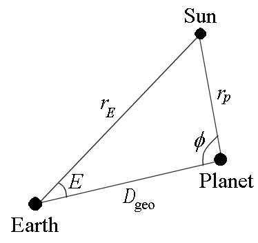
As shown in , elongation $E$ of a planet is the angular distance between the Sun and planet as seen from Earth. Phase angle $\phi$ of a planet is the angular distance between the Sun and Earth as seen from the planet. It follows from the law of cosine that
$$ \cos E = \frac{r_E^2 + D_{\rm geo}^2 - r_p^2}{2 r_E D_{\rm geo}} \ \ , \ \ \cos \phi = \frac{r_p^2 + D_{\rm geo}^2 - r_E^2}{2 r_p D_{\rm geo}} , \label{eq:ElongPhaseAng} $$where $r_E$ is the heliocentric distance of the Earth, $r_p$ is the heliocentric distance of the planet, and $D_{\rm geo}$ is the geocentric distance of the planet. This formula ignores the finite speed of light. In principle, ray tracing is needed if high precision is required. More accurate formulae are
$$ \cos E(t) = -\frac{\boldsymbol{r}_E(t) \cdot \boldsymbol{X}_p(t)}{|\boldsymbol{r}_E(t)| |\boldsymbol{X_p}(t)|} \ \ , \ \ \cos \phi(t) = -\frac{[\boldsymbol{r_E}(t_r)-\boldsymbol{r_p}(t)] \cdot \boldsymbol{r_p}(t)} {|\boldsymbol{r_E}(t_r)-\boldsymbol{r_p}(t)| |\boldsymbol{r_p}(t_r)|} , $$where the retarded time $t_r$ satisfies the equation $t_r=t-|\boldsymbol{r_E}(t_r)-\boldsymbol{r_p}(t)|/c$ and I ignore the Sun's motion with repsect to the solar system barycenter, aberration of light and gravitational deflection of light. The equation for the elongation is easy to calculate. It follows from
\begin{align} \boldsymbol{r_E} &= - r_E \left( \begin{array}{c} \cos \alpha_{\odot} \cos \delta_{\odot} \\ \sin \alpha_{\odot} \cos \delta_{\odot} \\ \sin \delta_{\odot} \end{array} \right) \\ \nonumber \cr \boldsymbol{X_p} &= |\boldsymbol{X_p}| \left( \begin{array}{c} \cos \alpha_p \cos \delta_p \\ \sin \alpha_p \cos \delta_p \\ \sin \delta_p \end{array} \right) \end{align}and the addition formula of the cosine function that
$$ \cos E = \sin \delta_{\odot} \sin \delta_p + \cos \delta_{\odot} \cos \delta_p \cos (\alpha_{\odot} - \alpha_p) . \label{eq:Elong} $$Accurate computation of $\phi$ is slightly more involved. However, elongation and phase angle are usually not quantities of great interest and so they are not calculated to high precision. I simply use equation \eqref{eq:ElongPhaseAng} and light-time correction is not done carefully for the three distances.
In the popup box for a planet, the elongation is displayed accurate to 0.1° and the direction of the planet relative to the Sun is indicated by either W or E. E means the planet is to the east of the Sun and W means it is to the west of the Sun. To be more specific, E means $\lambda_p-\lambda_{\odot} \gt 0$ and W means $\lambda_p-\lambda_{\odot} \lt 0$. Here $\lambda_p$ and $\lambda_{\odot}$ are the ecliptic longitude of the planet and the Sun, respectively. The difference $\lambda_p-\lambda_{\odot}$ is restricted to the range $[-\pi,\pi)$.
It can be shown (see e.g., Section 17.4 of Green, Spherical Astronomy, Cambridge University Press 1985) that the fraction of a spherical planet illuminated by the Sun is
$$ F = \frac{1+\cos \phi}{2} .$$In the popup box for a planet, $F$ is displayed to two decimal places. All planets are modelled as spheres, although the deviation from a sphere is substantial for Jupiter and Saturn. The value of $F$ for Jupiter, Saturn, Uranus and Neptune is almost 1 at all times because of their large distances from the Sun. The phase appearances of Mercury, Venus, and Mars are drawn in the popup box using the scalable vector graphics (SVG). The phase appearances of Jupiter, Saturn, Uranus and Neptune are not drawn since they are always almost full.
The apparent magnitude of a planet depends on its heliocentric distance $r_p$, geocentric distance $D_{\rm geo}$ and its phase angle $\phi$. The magnitude can be written as
$$ m = m_0 + 5\log_{10} \frac{r_p D_{\rm geo}}{{\rm AU}^2} + \Delta m(\phi) ,$$where $m_0$ is a constant and $\Delta m(\phi)$ is the variation of apparent magnitude as a function of $\phi$. The variation arises from the fraction of the planet illuminated and the property of diffuse reflection from the planet's surface/atmosphere. The function $\Delta m(\phi)$ is determined empirically and is listed in Table 10.6 of Explanatory Supplement to the Astronomical Almanac and errata. The table is reproduced below with errors corrected. The phase angle $\phi$ is in degrees.
| Planet | m0 | Δ m |
|---|---|---|
| Mercury | -0.60 | $0.0498 \phi - 0.000488 \phi^2 + 3.02\times 10^{-6} \phi^3$ |
| Venus | -4.47 | $0.0103\phi + 5.7\times 10^{-5} \phi^2 + 1.3\times 10^{-7} \phi^3$ for $2.2^\circ \lt \phi \lt 163.6^\circ$ |
| 0.98 | $-0.0102\phi$ for $163.6^\circ \lt \phi \lt 170.2^\circ$ | |
| Mars | -1.52 | $0.016\phi$ |
| Jupiter | -9.40 | $0.005\phi$ |
| Saturn | -8.88 | $0.044\phi - 2.6 |\sin e| + 1.25\sin^2 e$ |
| Uranus | -7.19 | $0.002\phi$ |
| Neptune | -6.87 | 0 |
Note that $\Delta m$ is undefined for Venus when $0^\circ \lt \phi \lt 2.2^\circ$ and when $170.2^\circ \lt \phi \lt 180^\circ$. In the popup box, the expression for $2.2^\circ \lt \phi \lt 163.6^\circ$ is used when $0^\circ \lt \phi \lt 2.2^\circ$ and the expression for $163.6^\circ \lt \phi \lt 170.2^\circ$ is used when $170.2^\circ \lt \phi \lt 180^\circ$.
Saturn's magnitude calculation is more complicated because its rings have significant contribution to Saturn's brightness. As a result, the terms $- 2.6 |\sin e| + 1.25\sin^2 e$ appear in the formula for Saturn's magnitude. Here $e$ is the Saturnocentric sub-Earth latitude, which determines the orientation of Saturn's rings seen from Earth. The value of $e$ is computed as follows. First compute the J2000.0 Ra and Dec of Saturn's north pole according to
$$ \alpha_0 = 40.^{\circ}589 - 0.^{\circ}036 T \ \ , \ \ \delta_0 = 83.^{\circ}537 - 0.^{\circ}004 T , $$where $T$ is the TT Julian century from J2000.0. Next compute the unit vector $\boldsymbol{e_3}$ pointing in the direction of Saturn's rotation axis:
$$ \boldsymbol{e_3} = \left( \begin{array}{c} \cos \delta_0 \cos \alpha_0 \\ \cos \delta_0 \sin \alpha_0 \\ \sin \delta_0 \end{array} \right) \label{eq:SaturnE3} $$Finally, the value of $\sin e$ is given by
$$ \sin e = \frac{\boldsymbol{X_S}\cdot \boldsymbol{e_3}}{|\boldsymbol{X_S}|} ,$$where $\boldsymbol{X_S}$ is Saturn's geocentric position.
Position of the Moon is calculated based on the ELP/MPP02 series. A JavaScript code is created based on the source code provided by the authors on this ftp site. The JavaScript code has been tested by comparing the results with those of the FORTRAN code on the ftp site. I find agreement to within 12 to 13 significant figures. The deviation is most likely caused by the accumulated roundoff error.
ELP/MPP02 is a semi-analytic solution for the lunar motion. There are parameters in the model that are fitted to either the lunar laser ranging (LLR) data or fitted to JPL's DE405/DE406 ephemerides. Parameters fitted to DE405/DE406 are used on our webpages. The deviation between the positions in ELP/MPP02 and DE405/406 is less than 3.5" in ecliptic longitude and 0.8" in ecliptic latitude over the time span from 3000 BCE to 3000 CE.
The full ELP/MPP02 series can be written in the form
\begin{align} V(T) &= W(T) + \sum_{i=0}^3 T^i \sum_j A^{(V)}_{ij} \sin\left[ \phi^{(V)}_{ij}(T)\right] \\ U(T) &= \sum_{i=0}^3 T^i \sum_j A^{(U)}_{ij} \sin\left[ \phi^{(U)}_{ij}(T)\right] \\ r(T) &= r_0 + \sum_{i=0}^3 T^i \sum_j A^{(r)}_{ij} \sin\left[ \phi^{(r)}_{ij}(T)\right] , \label{eq:Dmoon} \end{align}where $V$, $U$, and $r$ are the ecliptic longitude, ecliptic latitude, and geocentric distance of the Moon, respectively, $T$ is the TT Julian century from J2000.0, $W$ is the mean longitude of the Moon, $r_0$ is a constant. For the terms in the sum, $A^{(U)}_{ij}$, $A^{(V)}_{ij}$, $A^{(r)}_{ij}$ are constants. The phase angles $\phi^{(U)}_{ij}$, $\phi^{(V)}_{ij}$, $\phi^{(r)}_{ij}$ are linear functions of 13 angles $a_k$ $(k=1,2,\cdots, 13)$ related to the mean positions and orbital parameters of the Moon and solar system planets. The functions $W(T)$ and $a_k(T)$ are expressed as polynomial functions of $T$ up to and including $T^4$.
The full series involves about 36,000 terms. Since high accuracy is not needed for our use, I truncate the series by the following procedure:
- Choose four parameters $A^{(U)}_{\rm th}$, $A^{(V)}_{\rm th}$, $A^{(r)}_{\rm th}$ and $\tau$.
- Drop the terms in the series with $A^{(U)}_{ij} \lt A^{(U)}_{\rm th} /\tau^i$, $A^{(V)}_{ij} \lt A^{(V)}_{\rm th} /\tau^i$, and $A^{(r)}_{ij} \lt A^{(r)}_{\rm th} /\tau^i$.
It is clear that the smaller the parameters $A^{(U)}_{\rm th}$, $A^{(V)}_{\rm th}$, and $A^{(r)}_{\rm th}$, the closer the truncated series is to the original series. The parameter $\tau$ has a unit of time and is chosen to be 50 Julian centuries, which is the time span covered by the ELP/MPP02 series. Two sets of truncated series are created using two set of parameters. I call the two sets of truncated series ELP/MPP02L and ELP/MPP02C.
ELP/MPP02L is a low-precision series, created using $A^{(U)}_{\rm th}=A^{(V)}_{\rm th}=30''$, $A^{(r)}_{\rm th}=100$ km, and $\tau = 50$ Julian centuries. It is used for plotting the Moon on our star charts. The resulting series consists of about 40 terms. The accuracy of ELP/MPP02L is estimated by comparing it with the full series. Specifically, 10,000 random values of $T$ are chosen between -50 and 50. Values of $U(T)$, $V(T)$, and $r(T)$ at these times are computed for both the ELP/MPP02L series and the full series. I find that the maximum differences between ELP/MPP02L and ELP/MPP02 are $233''$ for $V$, $152''$ for $U$ and $352$ km for $r$. The root mean square of the differences are $47''$ for $V$, $33''$ for $U$ and $86$ km for $r$. This accuracy is sufficient for our plotting purpose.
ELP/MPP02C is created using $A^{(U)}_{\rm th}=A^{(V)}_{\rm th}=0.001''$, $A^{(r)}_{\rm th}=0.1$ km, and $\tau = 50$ Julian centuries. It is used in the calculation in the popup box. The resulting series consists of about 3750 terms. The accuracy of ELP/MPP02C is estimated in the same way as above. I find that the maximum differences between ELP/MPP02C and ELP/MPP02 over the time span $|T| \lt 50$ are 0.1" for $V$, 0.08" for $U$ and 1.9 km for $r$. The root mean square of the differences are 0.02" for $V$, 0.01" for $U$ and 0.4 km for $r$. The error of this truncated series is lower than the error of the apparent position caused by our ignoring the effect of polar motion.
Once $U$, $V$ and $r$ are computed, rectangular components of the geocentric position of the Moon with respect to the ecliptic and mean equinox of J2000.0 are obtained by taking into account precession and transformation from spherical to Cartesian coordinates. The procedure is described in the pdf document on the ftp site. Equatorial coordinates of J2000.0 mean equator and equinox are then computed by rotating the ecliptic coordinates by the angle $\epsilon_0=23^\circ 26' 21.406''$ (mean obliquity of the ecliptic at J2000.0) about the $x$-axis. The J2000.0 equatorial coordinates are basically the GCRS coordinates, apart from the tiny difference between these two systems caused by the 17-milliarcsecond offset, which I ignored. Light-time correction and aberration of light is implemented by first computing the geocentric distance $r(t)$ using equation \eqref{eq:Dmoon}. Then the retarded geocentric position is calculated by $\boldsymbol{X}(t_r) = \boldsymbol{X}(t-r(t)/c)$. Note that the retarded geocentric position includes both the light-time correction and aberration of light since $\boldsymbol{X}(t_r) = \boldsymbol{r_M}(t_r)-\boldsymbol{r_E}(t_r)$, where $\boldsymbol{r_M}$ and $\boldsymbol{r_E}$ are the barycentric position of the Moon and Earth, respectively. Light-time corrected geocentric position is $\boldsymbol{r_M}(t_r)-\boldsymbol{r_E}(t)$, and $\boldsymbol{r_M}(t_r)-\boldsymbol{r_E}(t_r)$ includes both light-time correction and annual aberration to first order in $v/c$ (see Section 7.2.3.5 of Explanatory Supplement to the Astronomical Almanac). The combined effect is called planetary aberration. Planetary aberration shifts the Moon's position by about $1''$. Hence the correction is ignored when using the low-precision ELP/MPP02L series.
GCRS position of the Moon is calculated using the low-precision ELP/MPP02L series. GCRS Ra and Dec are then calculated using $\alpha={\rm arg}(X+iY)$ and $\delta=\sin^{-1}(Z/r)$. The Moon can now be plotted on the GCRS charts: its canvas coordinates are given by equations \eqref{eq:stereographicXg}-\eqref{eq:mollweide}.
For the local star charts, the altitude $a$ and azimuth $A$ are required at the given location. First, the "of date" geocentric equatorial coordinates are computed by applying the precession matrix on $\boldsymbol{X}$. Since the Moon is close to the Earth, the geocentric parallax is significant, which is accounted for by computing its topocentric position using equations \eqref{eq:topoX}-\eqref{eq:topoCS}. The "of date" topocentric Ra and Dec is then calculated by $\alpha_{\rm topo} = {\rm arg}(X_{\rm topo}+iY_{\rm topo})$ and $\delta_{\rm topo}=\sin^{-1} (Z_{\rm topo}/D_{\rm topo})$, where $D_{\rm topo}=\sqrt{X_{\rm topo}^2 + Y_{\rm topo}^2 + Z_{\rm topo}^2}$ is the topocentric distance of the Moon. The hour angle is given by $H=t_s-\alpha_{\rm topo}$, where $t_s$ is the local apparent sidereal time (LAST). Next $a$ and $A$ are computed using equations \eqref{eq:aAFromHdel1}-\eqref{eq:aAFromHdel3}. Then the altitude is adjusted by the atmospheric refraction according to equation \eqref{eq:atmRefraction}. The Moon can now be plotted on a local star chart: its canvas coordinates are given by equation \eqref{eq:stereographicHor}.
In the popup box, the Moon's position is calculated using the higher precision ELP/MPP02C and with planetary aberration corrected. Geocentric position, topocentric position, altitude and azimuth are computed in the same way as described above when the time is outside the interval 3000 BCE-3000 CE. For times within the interval 3000 BCE-3000 CE, the J2000.0 positions include only the planetary aberration and geocentric parallax (for topocentric position). The apparent "of date" position, as well as altitude and azimuth, includes planetary aberration, precession, nutation and diurnal aberration of light. The calculations of precession and nutation are the same as those described in Section 14.4. For diurnal aberration, the vector $\boldsymbol{n'}$ is calculated by equation \eqref{eq:aberration} with $\boldsymbol{n}=\boldsymbol{X'}/|\boldsymbol{X'}|$, $\boldsymbol{X'}=\boldsymbol{X}(t_r)-\boldsymbol{X_L}$, and $\boldsymbol{\beta}=\boldsymbol{v_{\rm spin}}/c$. The geocentric position vector $\boldsymbol{X}_L$ of the location is calculated by equations \eqref{eq:XL} and \eqref{eq:topoCS}. The spin velocity $\boldsymbol{v_{\rm spin}}$ is calculated by equation \eqref{eq:vspin}.
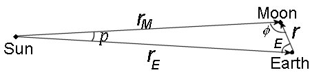
Elongation $E$ and phase angle $\phi$ can be calculated using equations similar to equation \eqref{eq:ElongPhaseAng}. However, it is easier to use equation \eqref{eq:Elong} to calculate $E$. For $\phi$, the Moon's heliocentric position $\boldsymbol{r_M}$ needs to be computed. As shown in , $\boldsymbol{r_M}=\boldsymbol{r_E}+\boldsymbol{r}$, where $\boldsymbol{r_E}$ is the heliocentric position of the Earth and $\boldsymbol{r}$ is the geocentric position of the Moon. It follows that
\begin{align} r_M^2 &= |\boldsymbol{r_E}+\boldsymbol{r}|^2 = r_E^2 + 2\boldsymbol{r}\cdot \boldsymbol{r_E} + r^2 \nonumber \cr &= r_E^2 - 2 r r_E \cos E+r^2 = r_E^2(1-2\sigma \cos E + \sigma^2) , \end{align}where $\sigma=r/r_E$ and I have used the fact that $\boldsymbol{r}\cdot \boldsymbol{r_E}=-r r_E \cos E$. The phase angle can be written as
$$ \cos \phi = \frac{r_M^2+r^2-r_E^2}{2rr_M} = \frac{\sigma - \cos E} {\sqrt{1-2\sigma\cos E + \sigma^2}} . \label{eq:ElongMoon} $$Since $r \approx 3.8\times 10^{5}$ km and $r_E\approx 1.5\times 10^8$ km, $\sigma \approx 2.5\times 10^{-3} \ll 1$. Hence $\cos \phi \approx -\cos E$ or $\phi \approx \pi - E$. This approximate relation between $E$ and $\phi$ can be understood geometrically. As seen in , when $r \ll r_M$ and $r \ll r_E$, the line joining the Moon and the Sun and the line joining the Earth and the Sun are nearly parallel. It follows from the Euclidean geometry that $\phi + E = \pi$ if the two lines were parallel. Since the two lines are nearly parallel, the relation is approximate. In fact, $\phi + E = \pi - p$, where $p$ is the angular separation between the Earth and Moon as seen from the Sun or the parallax of the Sun using Earth-Moon as the baseline. The difference between $\phi$ and $\pi - E$ is $p \sim r/r_E =\sigma \approx 2.5\times 10^{-3}$ radians or 0.15°. In the popup box, $\phi$ is computed according to equation \eqref{eq:ElongMoon} without using the approximation. The phase appearance of the Moon is drawn in the popup box using SVG.
The apparent magnitude of the Moon is calculated using the following approximate formula:
$$ m = -12.73 + 0.026 \phi + 4\times 10^{-9} \phi^4 + 5\log_{10}\left( \frac{r}{384400 {\rm km}}\cdot \frac{r_M}{1 {\rm AU}}\right) , $$where $\phi$ is the phase angle in degrees. This formula appears in Astronomy and the Limits of Vision by B.E. Schaefer, Vistas in Astronomy, 36, 311 (1993). It appears that this formula is used by JPL's Horizons website since their data closely match the formula. The JPL website states that when the phase angle <7° (within $\sim$ one day of full Moon), computed magnitude tends to be about 0.12 too small. That is, the formula does not account for opposition surge. It also does not account for the decrease in brightness when lunar eclipses occur.
The rise, set, and upper transit times of celestial objects, as well as the beginning and ending of twilight, are computed in the popup box, and on the rise/set page when the Rise and Set Times button on the local star chart page is clicked. This section describes the method and algorithm used to do the calculation.
The rise and set times of a celestial object are defined as the times when the upper limb of the object touches the horizon. Since the horizon depends on the observer's location, the rise and set times are different for different observers. The rise and set times are the times when the apparent topocentric altitude of the upper limb of the object is 0. The geocentric altitude of the object's center at the rise and set times is
$$ a_{rs} = p - \Delta a - s , $$where $p$ is the geocentric parallax, $\Delta a$ is the correction of the altitude due to atmospheric refraction and $s$ is the angular radius of the object. The atmospheric refraction term $\Delta a$ varies depending on the local conditions. For the Sun and Moon, $p$ and $s$ also vary slightly. Since the rise and set times are usually calculated to an accuracy of a couple of minutes, average values of $\Delta a$, $p$ and $s$ are used. The term $\Delta a$ is usually set to 34'. For the Sun, $p \approx 8.8''$, $s\approx 16'$ and so $a_{rs}=-50'$ for sunrise and sunset. For the Moon, $p\approx 57'$, $s\approx 15'$ and so $a_{rs}=8'$. For planets and stars, $p \ll \Delta a$ and $s \ll \Delta a$, and so I simply set $a_{rs}=-34'$.
Twilight is usually divided into three phases. The beginning and ending of the civil twilight are the times when the Sun's center is 6° below the horizon. When the civil twilight ends, the sky is dark enough for the brightest stars to be visible. The beginning and ending of the nautical twilight are the times when the Sun's center is 12° below the horizon. When the nautical twilight ends, the sky is so dark that the horizon is no longer visible. The beginning and ending of the astronomical twilight are the times when the Sun's center is $18^\circ$ below the horizon. They mark the beginning and ending of the night time. When the astronomical twilight ends, the faintest stars are visible (in regions with clear sky and no light pollution). Thus, $a_{rs}=-6^\circ$ for civil twilight, $a_{rs}=-12^\circ$ for nautical twilight and $a_{rs}=-18^\circ$ for astronomical twilight.
Transits are defined as the times when the object crosses the meridian, which are the times when the hour angle of the object is 0 or π. The $H=0$ transit is called the upper transit and the $H=\pi$ transit is called the lower transit.
Since the rise, set, and upper transit time calculation does not require high precision. Low-precision formulae for the positions of the Sun, Moon and planets are used. In addition, nutation, polar motion, aberration of light, and gravitational deflection of light by the Sun are ignored.
The rise and set times of stars can be computed relatively easily since their "of date" right ascension and declination do not change much during the course of a day.
It follows from equation \eqref{eq:aAFromHdel3} that
$$ \cos H = \frac{\sin a - \sin \delta \sin \phi}{\cos \delta \cos \phi} . \label{eq:cosH} $$Here $\delta$ is the "of date" declination of the star. Since $-1 \leq \cos H \leq 1$,
$$ -1 \leq \frac{\sin a - \sin \delta \sin \phi}{\cos \delta \cos \phi} \leq 1 $$or
$$ -\cos \delta \cos \phi + \sin \delta \sin \phi \leq \sin a \leq \cos \delta \cos \phi + \sin \delta \sin \phi . $$It follows from the addition formula of the cosine function that
$$ -\cos (\delta + \phi) \leq \sin a \leq \cos (\delta - \phi)$$which can be written as
$$ \sin (|\delta + \phi| - 90^\circ) \leq \sin a \leq \sin (90^\circ - |\delta -\phi|) . $$Since $|\delta|\leq 90^\circ$ and $|\phi| \leq 90^\circ$, $|\delta + \phi| - 90^\circ \in [-90^\circ, 90^\circ]$ and $90^\circ - |\delta -\phi| \in [-90^\circ, 90^\circ]$. By definition, the altitude $a \in [-90^\circ, 90^\circ]$. Since sine is an increasing function in $[-90^\circ, 90^\circ]$,
$$ |\delta + \phi| - 90^\circ \leq a \leq 90^\circ - |\delta -\phi| .$$The minimum and maximum geocentric altitude are
$$ a_{\rm min} = |\delta + \phi| - 90^\circ \ \ , \ \ a_{\rm max} = 90^\circ - |\delta -\phi| . $$The maximum altitude occurs when the hour angle $H=0^\circ$, which is the upper transit. The minimum altitude occurs when $H=180^\circ$, which is the lower transit.
For a given latitude $\phi$, there are stars with $a_{\rm min} \gt a_{rs}$. These stars are always above the horizon. They are called the circumpolar stars. A star is circumpolar if its declination satisfies the condition $\delta \gt 89^\circ 26' - \phi$ or $\delta \lt -(89^\circ 26' + \phi)$. Since $|\delta|\leq 90^\circ$, only the first inequality is relevant for northern hemisphere observers with $\phi \gt 34'$. Only the second inequality is relevant for southern hemisphere observers with $\phi \lt -34'$. Both inequalities are relevant only for observers very close to the equator with $|\phi| \lt 34'$.
There are also stars with $a_{\rm max} \lt a_{rs}$. These stars are always below the horizon. They are always invisible at the location. A star is always invisible if its declination satisfies the condition $\delta \lt -(90^\circ 34' - \phi)$ or $\delta \gt 90^\circ 34' + \phi$. Only the first inequality is relevant for observers with $\phi \gt 34'$. Only the second inequality is relevant for observers with $\phi \lt -34'$. For observers with $|\phi| \leq 34'$, there are no stars that are always invisible.
Thus the rise and set times are for stars that are not circumpolar and not always invisible. For these stars, the hour angle at the rise and set times are given by equation \eqref{eq:cosH} with $a=a_{rs}$:
$$ H_{\pm} = \pm \cos^{-1} \frac{\sin a_{rs} - \sin \delta \sin \phi}{\cos \delta \cos \phi} , $$When $H \gt 0$, the star is on the west side of the meridian. When $H \lt 0$, the star is on the east side of the meridian. Thus, the + sign is for the set time and - sign is for the rise time. The sidereal time at the rise and set times are given by
$$ t_{s\pm}= H_{\pm} + \alpha ,$$where $\alpha$ is the "of date" right ascension of the star. Over the course of a day, the sidereal time advances at a rate 1.00273781191135448 faster than the clock time based on UTC. To calculate the rise and set times at a given time zone, first calculate the sidereal time $t_{s0}$ at the midnight of the given time zone by
$$ t_{s0}={\rm LAST}(D_{Um},T(D_{Um})) = {\rm GAST}(D_{Um},T(D_{Um})) + \lambda , $$where $\lambda$ is the location's longitude, $D_{Um}=$ Julian UT1 date at midnight local time - 2451545.0, and $T(D_{Um})$ is the TT Julian century from J2000.0 at $D_{Um}$. In other words,
$$ T(D_{Um}) = \frac{D_{Um}}{36525} + \Delta T(D_{Um}) ,$$where $\Delta T$ is the difference between TT and UT1 described in Section 4. The Greenwich apparent sidereal time GAST is calculated using equations \eqref{def:UT1} and \eqref{eq:GAST}, and $\Delta T$ is calculated using the fitting and extrapolation formulae of Stephenson et al (2016) and Morrison et al (2021). The sidereal time $t_s$ at any later time of the date is given by $t_s=t_{s0}+1.00273781191135448 h'$, where $h'=24(D_U-D_{Um})$ is the number of hours past the local midnight. The local times at which the setting and rising of the star occur on a given date are
$$ h'_{\pm} = \frac{(H_{\pm} + \alpha - t_{s0})\ {\rm mod}\ 24^{\rm h}}{1.00273781191135448} . \label{eq:riseSetStars} $$Upper transit time is the time when the hour angle $H=0$. Hence
$$ h'_{\rm upper transit} = \frac{(\alpha - t_{s0})\ {\rm mod}\ 24^{\rm h}}{1.00273781191135448} . \label{eq:upperTransitStars} $$Note that equations \eqref{eq:riseSetStars} and \eqref{eq:upperTransitStars} imply that $h'$ can never be greater than 24/1.00273781191135448. This is because one sidereal day is 1/1.00273781191135448 days =23h56m4s and is smaller than 24 hours. Thus, if the rise/set/upper transit time occurs bewteen 0h and 0h03m56s, there will be another rise/set/upper transit occurring on the same day with $h' \gt 24/1.00273781191135448$. This occurs only once every year for each case and I ignore them.
The equations for the rise, set, upper transit times of the Sun, Moon and planets, as well as the beginning and ending of twilight, are still given by equations \eqref{eq:riseSetStars} and \eqref{eq:upperTransitStars}. The only difference is that the right ascension and declination for the Sun, Moon and planets change more rapidly over the course of a day. The two equations should be written more clearly as follows.
\begin{align} h'_{\pm} &= \frac{(H_{\pm}(\delta(h'_{\pm})) + \alpha(h'_{\pm}) - t_{s0})\ {\rm mod}\ 24^{\rm h}}{1.00273781191135448} \label{eq:riseSetPlanets} \\ \nonumber \cr h'_{\rm upper transit} &= \frac{(\alpha(h'_{\rm upper transit}) - t_{s0})\ {\rm mod}\ 24^{\rm h}}{1.00273781191135448} \label{eq:upperTransitPlanets} \end{align}These equations explicitly indicate that the rise/set/upper transit time depends on the values of α and δ at the rise/set/upper transit times. Since α and δ can no longer be considered as constants over the course of a day, the unknown rise/set/upper transit time appears on both sides of the equations. The equations may be solved iteratively. For the Sun and planets, α and δ change slowly over the course of a day. Treating them as constants will not cause an error of more than a few minutes, which is sufficient. However, the Moon moves rapidly over the course of a day and treating α and δ as constants will cause a large error.
There are two other complications. The time between two successive rise/set/upper transit times is one sidereal day for stars. This is not true for the Sun, Moon and planets. The most extreme case is the Moon, where the average time between two successive rise/set/upper transit times is 24 hours and 50 minutes. As a result, it is possible to have no rise/set/transit on a given day. Another complication is that at high latitudes, the rise and set times of the Sun, Moon and planets are sensitive to the change in declination when the object is close to being circumpolar or close to being invisible all day. These two complications make the iterative procedure difficult to implement. As a result, I use the algorithm described in Sections 3.7 and 3.8 of the book Astronomy on the Personal Computer by O. Montenbruck and T. Pfleger, 4th edition, Springer 2000 (corrected fourth printing 2009) to calculate the rise, set and transit times. The algorithm is based on quadratic interpolation.
The idea is to first calculate the hour angle $H(h')$ and altitude $a(h')$ at local times 0h, 1h, ..., 24h, i.e. at $h'=0, 1, ..., 24$. Divide the day into 12 intervals: [0h, 2h), [2h, 4h), ..., [22h, 24h). Next values of $H(h')$ and $a(h')$ in each of the 12 intervals are approximated by a quadratic interpolation. Therefore, there are approximate analytic formulae for $H(h')$ and $a(h')$ throughout the day and the rise, set, and upper transit times are then solved by the equations $a(h')=a_{rs}$ and $H(h')=0$ using analytic expressions.
The procedure for the rise, set, beginning and ending of twilight works as follows. For $h'$ in a particular time interval, define
$$ x = h'-h'_0 \ \ \ , \ \ \ y = \sin [a(h')] - \sin a_{rs} ,$$where $h'_0$ is the mid-point of the time interval. Thus $x\in [-1,1)$ and $y=0$ at the rise and set times. Next, fit a quadratic curve $y(x)=c_2 x^2+c_1x+c_0$ in the interval based on the three values of $y$ at $x=-1$, 0 and 1:
$$ y_- = y(-1)=c_2-c_1+c_0 \ \ , \ \ y_0=y(0)=c_0 \ \ , \ \ y_+=y(1)=c_2+c_1+c_0 . $$Values of $c_0$, $c_1$, and $c_2$ are easily solved to give
$$ c_2 = (y_+ + y_-)/2 - y_0 \ \ , \ \ c_1 = (y_+ - y_-)/2 \ \ , \ \ c_0=y_0 . $$The quadratic equation $y(x)=0$ has roots if $c_1^2-4c_0c_2 \geq 0$ and the roots are given by $x_{\pm}=(-c_1\pm \sqrt{c_1^2-4c_0c_2})/(2c_2)$. The quadratic function $y(x)$ reaches an extremum at $x_m=-c_1/(2c_2)$. However, the function $y(x)$ only applies in the interval $x\in [-1,1)$. In general, there can be 0, 1 or 2 roots in the interval [-1,1). Let's consider these three cases.
Case 1: There is no root in the interval [-1,1). No rising and setting occurs in this time interval. Move on to the next time interval.
Case 2: There is one root, $x_1$, in the interval [-1,1). Either rising or setting occurs in this time interval at $h'=h'_0+x_1$. It is rising if $y_- \lt 0$ and $y_+ \gt 0$; it is setting if $y_- \gt 0$ and $y_+ \lt 0$.
Case 3: There are two roots, $x_1$ and $x_2$, in the interval [-1,1). Suppose $x_2 \gt x_1$. Then rising and setting both occur in this time interval and the extremum $x_m=(x_1+x_2)/2$ is also inside this interval. If $y(x_m) \gt 0$, the object rises at $h'=h'_0+x_1$, reaches a maximum altitude at $h'=h'_0+x_m$ and sets at $h'=h'_0+x_2$. This could happen when the object is close to being invisible and it only spends less than two hours above the horizon near its upper transit. If $y(x_m) \lt 0$, the object sets at $h'=h'_0+x_1$, reaches a minimum altitude at $h'=h'_0+x_m$ and rises at $h'=h'_0+x_2$. This could happen when the object is close to being circumpolar and it only spends less than two hours below the horizon near its lower transit.
By going through all the 12 intervals, the rise and set times can be found. For the upper transit time, the calculation is done in a similar way. I set $y = H(h')$ in this case. Care must be taken when calculating the roots of $y=0$. If $\alpha(h')$ and $\delta(h')$ are constants, $y$ will be a linear function of $x$ and so $c_2=0$. For the Sun and planets, $\alpha(h')$ and $\delta(h')$ are nearly constants and so $y(x)$ is close to being a linear function with $|c_2|\ll 1$. One of the roots is close to $-c_0/c_1$ and the other is close to $-c_1/c_2$. The root close to $-c_0/c_1$ can be calculated using the expression $x_1=-2c_0/D$ and the one close to $-c_1/c_2$ can be calculated using $x_2=-D/(2 c_2)$, where $D=c_1+\sqrt{c_1^2-4c_0c_2}$ if $c_1 \gt 0$ and $D=c_1-\sqrt{c_1^2-4c_0c_2}$ if $c_1 \lt 0$. Since $|c_2|\ll 1$, it is almost certain that the root close to $-c_1/c_2$ is outside the interval [-1,1). Only the root close to $-c_0/c_1$ has a chance of being inside the interval [-1,1). Normal celestial objects are not moving fast enough for there to be two upper transits occurring in a two-hour time interval and so Case 3 will never occur.
The algorithm described above has been tested on stars and the times computed match those calculated using equations \eqref{eq:riseSetStars} and \eqref{eq:upperTransitStars}. The difference is at most one minute. As in the case of stars, on rare occasions there could be more than one rise/set/upper transit times for the Sun and planets on a day. The algorithm described above can find all of them, but only the earliest time is reported in the popup box and on the rise/set page.
Notes
[Barbier] More constellation boundary data can be found on Pierre Barbier's constellation boundary page.
[Cal_Note] It's the standard convention to switch from Julian to Gregorian calendar after October 4, 1582 and use proleptic Julian calendar before 8 CE in astronomical computation. However, this convention is not necessarily followed elsewhere, especially in computer software. Apparently some software use Gregorian calndar before October 15, 1582. This is known as the proleptic Gregorian calendar. The case of Unix's (and Linux's)
calfunction is particularly strange. It switches from Julian to Gregorian calendar after September 2, 1752, by which time it was necessary to correct by 11 days. This was the date when the Great Britain and its colonies adopted the Gregorian calendar. When you typecal 1752in a Unix/Linux/MacOS terminal, you will see that the date following September 2 is September 14.[Gaia] Actually, accurate data are available now thanks to the Gaia mission, but I haven't incorporated them yet.
[Github] I have created this GitHub repository to provide C++ subroutines to implement the ELP/MPP02 series, construct truncated series, and generate JavaScript code to calculate the truncated series.
[GPS] Perhaps the best example to illustrate this effect is the Global Positioning System (GPS). The GPS navigation relies on comparing the times of emission and reception of radio waves from GPS satellites to the user. To achieve a navigation accuracy of 15 meters, time throughout the GPS system must be known to an accuracy of 50 nanoseconds, which simply corresponds to the time required for light to travel 15 meters. However, the GPS satellites are moving at 14,000 km/hr at an altitude of about 20,000 km from the ground. The combined effect of special and general relativistic time dilation results in the satellite clocks advancing faster than a clock on the ground by about 38.3 microseconds per day, or 26.6 nanoseconds per minute. If this effect is not taken into account, GPS would fail in its navigational functions within 2 minutes. See Clifford Will's article "Einstein's Relativity and Everyday Life" for a more detailed description.
[IAU_B2] IAU 2006 Resolution B2 recommends that the BCRS definition is completed with the following: "For all practical applications, unless otherwise stated, the BCRS is assumed to be oriented according to the ICRS axes. The orientation of the GCRS is derived from the ICRS-oriented BCRS."
[IERS conventions] IERS Conventions 2010, edited by G. Petit and B.Luzum.
[Kaplan] G.H. Kaplan, The IAU Resolutions on Astronomical Reference Systems, Time Scales, and Earth Rotation Models, U.S. Naval Observatory Circular No. 179 (Washington: USNO), 2005
[Urban & Seidelmann] S.E. Urban and P.K. Seidelmann. Explanatory Supplement to the Astronomical Almanac, 3rd edition, University Science Books, Mill Valley, California (2013). Errata: https://aa.usno.navy.mil/downloads/exp_supp_errata.pdf